CVA credit valuation adjustment

CVA (Credit Valuation Adjustment) = market value of counterparty credit risk

Recent high levels of CDS spreads make CVA an important quantity in valuation of OTC derivatives.

Before, the same interest rate swap would have the same value for two different counterparties, while now , the same swap would have different price , depending on credit rating of the bank’s client and portfolio of exiting derivatives.

what is CVA?

CVA= (value portfolio taking into account counterparty credit risk)- (value of risk-free portfolio).

in simplified form it’s equivalent to Exposure to default * probability of default * Loss given default

Exposure to default (EAD) = non-negative market value of portfolio at time of default , usually is calculated using monte carlo techniques
probability of default could be estimated from market CDS prices (or OAS spread of bonds)
LGD is based on expected recovery in case of counterparty default (in simple case it’s just (1-Recovery) Recovery is usually set to 40% )
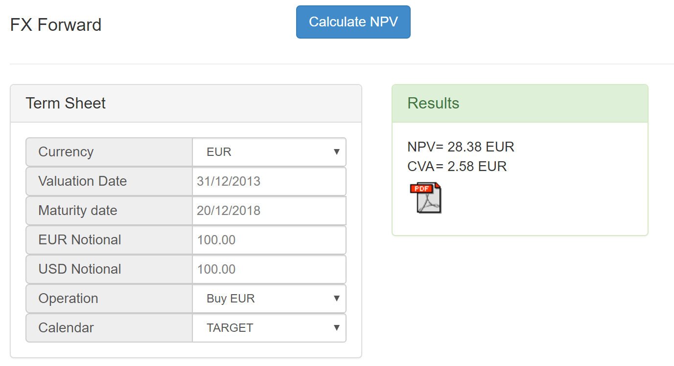
example

let’s take interest rate swap with notional 100 euros , maturity in 5 years , coupon of 1% (near market)
it’s risk-free price would be around 0.36 euros
when counterparty is tier-1 European bank counterparty CVA would be 0.10 eur (supposing we have no other OTC derivatives with Santander)
while when counterparty is tier-2 bank CVA would be around 0.25 eur , therefore Credit Risk adjusted value almost doubles the original risk free fair-value
(calculations of sept 2012, for spanish banks)

deploying CVA

Deploying CVA implied changes in valuation systems, introduction of new systems of CVA pricing and risk-management, and in appropriate case, creation of CVA desk

CVA desk

For managing and aggregating efficiently Counterparty risk many banks have created CVA desk: trading desk which centralizes managing of Counterparty Credit Risk (CRR) for all other trading desks (equity OTC derivatives desk, fx OTC derivatives desk etc).CVA desk charges a fee for this management . and these fees normally would be passed onto banks clients. once all these risks a aggregated CVA desk hedges the exposure with CDS contracts or Credit indices contracts (iTraxx for example)

possible deploing difficulties

CVA required very complicated calculations which needs powerful IT systems.It’s of great importance especially for Front Office which need to get CVA charge in real time (incremental CVA).Normally this would require highly parallelized grid systems.

Another heavy calculation step is obtaining CVA greeks which wold also require grid system.

Problems can arise while integrating 3 systems into one – portfolio data with each client, real time market data, netting agreements with clients)

For probabilities of default calculations one needs liquid CDS market which only exists for some counterparties, otherwise CDS proxies are needed.

wrong-way risk arises when counterparty exposure is highly correlated with CDS spread, for example in case of short CDS position.in this case one needs to complicate the calculations with correlations beween credit risk and other market variables.

also CVA calculation system would need to take into account Basel III requirements as some hedges are not eligible under Basel 3.

financial impact?

during financial crisis almost 70% of CCR losses were attributed to CVA losses and only 30% were attributed to actual defaults (Basel comitee)

recently JP Morgan declared losses of over 2bn$ in it’s division responsible for CVA hedging
goldman sachs could have a overall negative exposure to AIG thanks to it’s CVA desk

CVAvaluation systems
global banks have spent over 900MM$ in systems supporting CVA

Posted in OTC derivatives valuation Tagged with:

OIS discounting

Swap valuation with OIS discounting

OIS-discounting (from Overnight Indexed Swap)
is a derivatives valuation method considering multiple curves (and not one as before) for discounting and for projecting future cash flows.It’s used for collateralized derivatives.

CSA (Credit Support Annex)
its a contract (read “credit support”=collateral) which defines collateral management between counterparties of the contract. OIS discounting is the same as CSA-discounting.

Derivatives Valuation Changes

After the credit crunch of 2008 euribor rates cannot be considered as risk-free , because of the substantial spread between EONIA and Euribor swap (it used to be few bp before)
So, more and more swaps are getting collateralized now , and the interest rate which is paid on collateral is generally EONIA rate (for EUR cash collateral, for USD cash collateral it would be Fed Funds rate).
Because of this , the cashflows of the derivative should also be discounted with corresponding OIS rate.
from 2010 on LCH.Clearnet (major interest rate swap clearing house) has adopted its valuation method to OIS discounting.

Why negotiate swaps with collateral?
Dodd Frank act in the US and EMIR in Europe require that all eligible swaps be collateralized. In the same line BASEL III creates incentives for financial institutions to collateralize swaps (they would need less regulatory capital)

example

lets take a 5 year fixed-floating swap 100 euros notional , with 5% (out of the market) fixed rate and floating rate Euribor 6m (MTM of the swap about 19 euros)
with old method future cashflows are discounted and projected using the same euribor6m-based curve.
with OIS-discounting the cashflows are discounted using EONIA curve and projected using euribor6m-based curve(adjusted for EONIA discounting, which would slightly change the forward euribor rates)
difference between old and OIS discounting would be around 20 cents.

for at he market swaps the difference would be 0.
[calculations for sept 2012]

Deployment

In order to change to OIS-discounting one needs to make changes in legacy derivatives valuation systems – Front Office, Middle office , risk management, and collateral management systems.basic change is to introduce multiple curves for pricing and relevant changes for forward curves constructions.

difficulties in implementation

In the actual CSA (credit support annex) has many optionalities for both parties to post collateral (for example different currencies, different thresholds) which makes that every contract is unique.
The optionality for posting collateral in different currencies makes it a quanto product.Also some currencies still don’t have a liquid OIS-based swaps.

What is a financial impact?

several big banks has already published financial impact of OIS-discounting. bnp paribas has registered negatives impact of 108 millions EUR (2011),
crédit agricole 120 millions ,while some other banks have registered positive impacts , like Morgan stanley +176 M$ (2010),similar impact on RBS.
The sign of impact depends on the direction of the swap book of the institution.
MTM impact is material for legacy ,off-market , and forward starting swaps.
As a consequence it quite affects asset-swaps with euribor leg.

instruments:

apart from vanilla swap effect is big on instruments with euribor leg (this leg must be revalued).it also introduces dependance on EUrobor-EOnia spread to instruments which only were dependent on Euribor rates.
In general the difference is proportional on EONIA-euribor spread.
apart from the banks there is a big impact on insurers which have highly directional books

Posted in OTC derivatives valuation Tagged with: ,

how to value interest rate swap with 2 curves with QuantLib C++ (quantlib swap example)

example of interest rate swap derivative valuation in c++ with quantlib.
for quantlib excel valuation see http://www.pricederivatives.com/en/amortizing-swap-valuation-excel-example/

maturity: 20 nov 2022
nominal: 1M
init date: 20 nov 2012
floating leg pays: Euribor 3m + 2% every 3 months
fixed leg pays:4% anually

calendar: TARGET
day counting convention fixed leg: 30/360
day counting convention floating leg: Actual/360

market data :

last fixing for Euribor 3m : 1%

for discounting we’ll use Eonia curve (could be obtained from reuters or bloomberg)
(here we’ll use faux market data)

[date] [discount factor]

31 Dec 2013 0.99
31 Dec 2024 0.80

for euribor forwards calculation we’ll use projecting curve (euribor 3m):

[date] [discount factor]

31 dec 2013 0.999
31 dec 2024 0.89

QuantLib swap example c++ code for valuation of this swap contract for 31/dec/2012 :

#include <ql/quantlib.hpp>

using namespace std;
using namespace QuantLib;
using namespace boost;

int main()
{
vector<Date> dates; 
vector<DiscountFactor> discountFactor; 

Date valuationDate(31,December,2012);
Settings::instance().evaluationDate()=valuationDate;

dates.push_back(valuationDate); discountFactor.push_back(1.0); 
dates.push_back(Date(31,December, 2013));  discountFactor.push_back(0.99); 
dates.push_back(Date(31,December, 2024));  discountFactor.push_back(0.80); 
shared_ptr<YieldTermStructure> forwardCurve(new InterpolatedDiscountCurve<LogLinear>(dates,discountFactor,Actual360())); 

discountFactor.pop_back();discountFactor.pop_back();

discountFactor.push_back(0.999);
discountFactor.push_back(0.89);

shared_ptr<YieldTermStructure> oisCurve(new InterpolatedDiscountCurve<LogLinear>(dates,discountFactor,Actual360())); 

Handle<YieldTermStructure> discountingTermStructure(oisCurve);
Handle<YieldTermStructure> forwardingTermStructure(forwardCurve);

Real nominal = 1000000.0;
Date previousResetDate(20,November,2012);
Date maturity(20,November,2022);
double spread = 0.02;
double fixedRate=0.04;

shared_ptr<IborIndex> euribor(new Euribor(3*Months,forwardingTermStructure));
euribor->addFixing(euribor->fixingDate(previousResetDate),0.01,true);
		
VanillaSwap::Type swapType = VanillaSwap::Payer;

Schedule fixedSchedule(previousResetDate, maturity,1*Years,
                               TARGET(), ModifiedFollowing,ModifiedFollowing,
                               DateGeneration::Forward, false);

Schedule floatSchedule(previousResetDate,maturity,3*Months,
                               TARGET(),ModifiedFollowing ,ModifiedFollowing,
                               DateGeneration::Forward, false);
        
VanillaSwap swap(VanillaSwap::Payer, nominal,fixedSchedule, fixedRate, Thirty360(),
            floatSchedule, euribor, spread,Actual360());
     
shared_ptr<PricingEngine> swapEngine(new DiscountingSwapEngine(discountingTermStructure));

swap.setPricingEngine(swapEngine);
       
double res=swap.NPV();

}


Posted in quantlib Tagged with: ,

How to value FX forward pricing example

FX forward

Definition

An FX Forward contract is an agreement to buy or sell a fixed amount of foreign currency at previously agreed exchange rate (called strike) at defined date (called maturity).

FX Forward Valuation Calculator

fx forward

fx forward

FX forward example

  1. trade date : 1/oct/2012
  2. maturity date: 1/oct/2013

on maturity date A will buy 100 USD at exchange rate EURUSD 1.23

FX forward pricing

What market data do we need?

  1. forward points
  2. EUR discount curve

Forward points for 1 month represent how many basis points to add to current spot to know the forward EURUSD exchange rate
(for valuation date of today could be found on page fxstreet)

for example if forward points for EURUSD for 1 month is 30 and eurusd spot for valuation date is 1.234 then
the forward rate EURUSD for valuation date+ 1 month would be $$1.234+30/10000=1.237$$

FX forward valuation algorithm

  1. calculate forward exchange rate in euros: Forward in dollars=spot+Forwardpoints/10000 , Forward in Euros=1/ForwardInDollars
  2. caclulate net value of transaction at maturity: NetValue=Nominal*(Forward-Strike)
  3. discount it to valuation date with EUR discount curve: NPV=DiscountFactorEUR(maturity)*NetValue

FX forward example valuation:

valuation date: 1/oct/2012

market data:

forward FX points EURUSD 12months = 100

discount factor EUR (1/oct/2013) = 0.9

Spot EURUSD (1/oct/2012) = 1.234

1) calculate FX Forward for 12 months maturity:

Forward 12m EURUSD=1.234+100/10000  = 1.244

Forward USDEUR = 1/1.244=0.8039

2) calculate value at maturity:

strike in EUR = 1/1.23 = 0.813

Value(maturity)=100 (0.8039-0.813)=-0.91496 EUR

3) descount value to valuation date

NPV= 0.9*(-0.91496)=-0.82346 EUR

Excel calculation example (you can edit white cells):

Excel offline file using quantlib addin:
FX forward valuation example EURUSD using quantlib excel addin

Posted in OTC derivatives valuation Tagged with: , , ,

how to install python quantlib windows

Here we’ll show two ways to install quantlib package for python under windows [under unix/linux just install quantlib-python package from your favorite package installer]

first way (somewhat lengthy) is to compile it youself
second and easy way is install it from winpython package (see below)

Compile and install

you’ll need visual studio 2008 because python is compiled with it

install python 2.7

download quantlib 

download quantlib-swig (can be for linux distribution, for example for debian)

download boost 1.47 version is ok

extract all this to directory without spaces in name [there’s a bug in python script if ther’re spaces

modify enviroment variables:

INCLUDE = path to boost

QL_DIR = path to quantlib

build quantlib

go to swig/python dir

execute:

python setup.py build --compiler=msvc

python setup.py install

if you have several visual studio installations (VS 2012 and VS 2008 for example) you’ll need to run this from visual studio command promt (and indicating full path to python.exe)

Easy way with WinPython

install WinPython

download Quantlib package for your platform from here

run winpython control panel .exe
and point to downloaded quantlib package , Install

to use QuantLib run

from QuantLib import *

Posted in quantlib

simple example Libor Market Model (BGM)

Libor Market Model is a model where Libor forwards have log-normal distribution in their’s respective probability measures (called T-measure)

example of Libor Market Model with just 2 forwards:

$$ P_3(t)$$ is a price at time t of zero-coupon bond paying at $$T_3$$

$$ F_{T_1->T_2}(t)$$ is Libor forward [fixing $$T_1$$, maturity $$T_2$$]

Libor Market Model

Libor Market Model

lets take a numeraire=bond $$P_3(t)$$

in LMM forward $$ F_{T_2->T_3}(t)$$ is martingale i.e. it has the following dynamics in the $$P_3(t)$$ measure de:
$$ dF_{2->3}(t)=F_{2->3}(t) \sigma_2 dW_2(t) $$
from this dynamics we could deduce the Black formula for caplet $$T_2->T_3$$
[this is the formula which is used by market , that why Libor market model]

forward $$F_{1->2}$$ is not a martingale anymore and will have a drift

$$ dF_{1->2}(t)=F_{1->2}(t) ( drift(t) + \sigma_1 dW_1(t) )$$

Browinan motions $$W_1(t) and W_2(t)$$ are usually correlated

$$ dW_1(t)dW_2(t)=\rho dt $$

this drift(t) can be calculated (idea : $$ (1+\delta F_{1->2} ) (1+\delta F_{1->2}) $$ must be martingale )

once we have a formula for drift we could simulate the simultanious dynamics of both forwards with monte-carlo and calculate any payoff dependend on these forwards

– long jumps

as drift depends on forwards to simulate long jumps first project forwards with F(0) values , get F(T) then use 0.5(F(0)+F(T)) as constant forwards in drift to get F(T) second time

Posted in OTC derivatives valuation Tagged with:

why discount collaterized swaps with EONIA?

the collateral at every moment must coincide with value mark-to-market of swap

let’s take as a example simple swap with just one cashflow , which pays 100 euros at time T [it has no variable leg]

at time T swap’s value is 100 euros
so collateral value is also 100
at time T-1 (previous day) how much collateral we have to put?
if collateral is in EUR and grows with overnight EONIA rate
we must put 100 euros (=value of cashflow) decounted with EONIA rate
but as collateral coincides with MTM of derivative the cashflow must be discounted with the same rate

another example

if swap is in EUR but the collateral is in USD we still have to discount the derivative with OIS rate (usd fed funds)

Posted in OTC derivatives valuation Tagged with: ,

how to caclulate fair value of interest rate swap

how to caclulate fair value of interest rate swap

Online Interest Rate Swap Calculator

tipical example of interest rate swap contract between A and B:

example of swap

init date: 1/5/2012
maturity date: 1/5/2014
notional: 1 000 000 Eur
payments: annually
day counting convention: Actual/360
calendar: TARGET
bad day convention: Modified Following
A pays: fixed rate 4%
B pays: Euribor 12m

this contract can be represented by following cashflow diagram:

swap cashflows

swap cashflows

Euribor rates generally are fixed at the beginning of the period (in our case one year before payment)

how to calculate fair value?

valuation algorithm

  1. calculate net cashflow at every paydate
  2. discount each cashflow to valuation date
  3. sum all net discounted cashflows
payment 1 (1/5/2013)
A pays 4% on 1 000 000 = 40000 eur
we must multiply this quantity by year fraction with base Act/360 = frac(1/5/2012 -> 1/5/2013) = 1.014
so finally A pays 40000*1.014=40560 eur
B pays euribor 12m fixed on 1/5/2012 [  1.321 % ] i.e. B pays 1000000*0.01321*1.014 = 13394 eur
net pay1 = 40560 – 13394 =  27166 eur
this cashflow we must discount with EUR discount curve caclulated on 31/12/2012
suppose that discount factor for 1/5/2013 is 0.9
so discounted cashflow 1 will be 27166*0.9 = 24449 eur
payment 2 (1/5/2014)
A pays 4% on 1 000 000 = 40000 eur
multiply it by year fraction 1.014
A pays 40000*1.014=40560 eur
B pays euribor 12m fixed on 1/5/2013
this date is in the future so we must estimate it (=calculate euribor forward) with forwarding yield curve Euribor 12m on 31/12/2012
we can calculate this forward by formula:
$$ F= \frac{1}{YearFrac(1/5/2013 -> 1/5/2014)}(\frac{ DF(1/5/2013)}{DF(1/5/2014)}-1) $$
here the year fraction is calculated with the convention of the discounting curve  (suppose its the same act/360 convention)
if DF(1/5/2013)=0.8
and DF(1/5/2014)=0.85
then B would pay 1000000*0.058*1.014 = 58812 eur
net pay1 = 40560 – 58812 =  -18252 eur
this cashflow we must discount with the discounting yield curve with reference date 31/12/2012
suppose that discount factor( 1/5/2014)= 0.7
so discounted cashflow1 is -18252*0.7 =-12776.4 eur
So , this swap’s fair value on 31/12/2012 is -12776.4 eur
Posted in OTC derivatives valuation Tagged with:

how to construct yield curve in quantlib [ quantlib yield curve example ]

bloomberg or reuters can give you already bootstrapped curve in format [date] [discount factor]

here we’ll show a quantlib yield curve example construction

yield curve normally is used for getting a discount factor for a given date and for calculating euribor forwards

here we’ll show code snippet with quantlib which show show to use these functions

market date example:

valuation date: 31/dec/2012

[date] [discount factor]
30/12/2013 0.99
30/12/2014 0.98

we’ll calculate discount factor for 25/june /2013 and euribor forward 6m for the same date

#include <ql/quantlib.hpp>

using namespace std;
using namespace QuantLib;
using namespace boost;

int main()
{

vector<Date> dates; 
vector<DiscountFactor> discountFactor; 

Date valuationDate(31,December,2012);

dates.push_back(valuationDate); discountFactor.push_back(1.0); 

dates.push_back(Date(30,December, 2013));  discountFactor.push_back(0.99); 
dates.push_back(Date(30,December, 2014));  discountFactor.push_back(0.98); 

shared_ptr<YieldTermStructure> curve(new InterpolatedDiscountCurve<LogLinear>(dates,discountFactor,Actual360())); 

//discount factor
Date datex(25,June,2013);
double discount=curve->discount(datex);

//euribor forward
Period period(6*Months);
boost::shared_ptr<IborIndex> euribor(new Euribor(period));
double forward6m=curve->forwardRate(datex,period,curve->dayCounter(),QuantLib::Compounding::Simple);

}


Posted in quantlib

monte carlo method in finance

whats is monte carlo method in finance?

its a numerical method for calculating option’s price.
it consist in generating many possible scenarios and calculate average.

example – call option

suppose Black-Scholes (lognormal) dynamics for underlying stock S. suppose interest rate and dividends are 0:

$$dS=S \sigma dW_t $$
$$dW_t$$ is standard browinian motion

1) discretize the equation with just one time step:
$$ S_1=S_0+S_0\sigma \epsilon $$
where
$$\epsilon$$ is a standard gaussian

2) generate N random gaussian numbers $$ \epsilon_1,\epsilon_2,\epsilon_3,..\epsilon_N $$
3) calculate $$S_1$$ for every $$\epsilon$$
so we’ll have $$ S_1(\epsilon_1) , S_1(\epsilon_2) ,.., S_1(\epsilon_N) $$
4) calculate payoff of the option for every $$ S_i$$
call payoff is$$ (S_1(\epsilon_1)-K)^+ $$
5) calculate option’s price as average of these payoffs

if interest rates are not 0 we’d need to change S dynamics and discount payoff with corresponding discount factor

Posted in OTC derivatives valuation