What are crypto derivatives?

What are crypto derivatives?

Crypto derivatives are financial products where payoff (cashflow you get at maturity) is a formula of a price of crypto coin or crypto-related index (e.g. BTC price or BTC volatility index) . Crypto derivatives can be listed on exchanges (e.g. deribit or CME) or OTC ( over-the-counter) which are used primarly by institutions. Here we will consider only listed crypto derivatives.

What are the three common types of crypto derivatives?

the most traded crypto derivatives are the following:

1. perpetual swaps.

Crypto perpetual swap is the most traded crypto derivative.
perpetual swaps( also called perpetual futures, or perps) are most similar to usual CFD (contract for difference) products usually provided by common FX brokers. Holding a perpetual swap is more or less equivalent of holding underlying coin with leverage. perpetual swaps do not have a maturity date.
this is the most liquid type of crypto derivative.
example

2. crypto futures

Crypto futures have a maturity date on which you receive payoff of (S_T-S0) e.g. difference between price of underlying coin on maturity date and price of that underlying coin on purchase date. this is roughly equivalent of holding underlying coin with leverage, with an obligation to settle contract on maturity date (unlike perps)
example

3. crypto options

Crypto options also have a maturity date on which you receive payoff of max(S_T-K,0) e.g. you receive
difference between price at maturity date and strike price of the option , but only if it is positive.

The example formula of max(S_T-K,0) is for the call option . for put options formula payoff is max(K-S_T,0) e.g. you receive positive part of Strike minus maturity price of the underlying coin.

crypto options can be linear and inverse. inverse crypto options (e..g original crypto options listed on deribit) will pay payoff in crypto , while linear option will pay payoff in stablecoin (e.g. USDC/USDT)
margin of linear options is usually also calculated in stablecoin , while inverse margin is usually in underlying crypto coin.

how crypto derivatives are used:

crypto derivative usage is similar to that of financial derivatives: speculation or hedging and market making.

Example usage of speculation:

trader speculates that BTC price will be higher on 31 december than today.
he can buy (=go long) BTC perp, and wait 31 december. if price went up and was always higher than liquidation price up until 31 december . he will receive the difference between price on 31 december and purchase price multiplied by leverage. during lifetime of perpetual swap he would pay/receive funding payments (every 8 hours or 1 hour, depends on exchange) .

in case he does not want to bother with funding payments, he can instead buy crypto futures with maturity date of 31 december. in this case there are no funding payments and he would receive (S_T-S0)* leverage on maturity date, conditional on BTC price always being above his liquidation price.

in case he does not want to bother with the risk of being liquidated due to leverage, he can instead buy crypto call option. in that case there are no funding payments, and there BTC price can dip below any threshold before 31 december, he would still receive the payoff of max(St-K,0) on the maturity date.
this convenience is not free and on going long /buying the call option he has to pay option premium.
in case of perpetuals and futures, there is no any option premium to pay. (e.g. there is no cashflow at purchase time)

in case he speculates BTC price will go down, he can 1.sell perptual (= go short) 2. sell BTC futures 3. buy put option .

example usage of hedging:

Let’s say BTC miner wants to secure dollar profit of mining bitcoin for Year end of 31december. in that case upon receiving the BTC mining reward, he can enter short position on inverse BTC future with the maturity date of 31 december. if he uses his newly mining BTC reward as a margin, without using leverage, he can guarantee the BTC price as of the date of mining . even if BTC price went down after mining, the futures payoff will compensate for the difference. in case BTC price goes up , miner will not benefit from that appeciation. in case he does want to profit from possible BTC appreciation before 31 december, instead of selling futures contract he can buy put option. in this case if BTC price is lower on 31 december, long put option will compensate for it, but in case BTC price is higher, put option will expire worthless , but miner can sell his original BTC reward with higher price.

Crypto derivatives vs traditional financial derivatives

The difference with traditional derivatives is that in crypto settlement on crypto exchanges has usually much shorter time (seconds) instead of days. Traditional finance exchanges usually do not offer perpetual swaps and inverse instruements. The disadvanage of using crypto exchanges is that usually they have higher counterparty risk than traditional equity derivatives exchanges.

Another difference is the interest rate. in traditional financial derivatives pricing one can use liquid interest rate markets to determine interest rate used in formulas to price options and futures. in crypto there is no yet liquid interest rate market, thus crypto exchanges usually calculate implied volailities and other greeks using 0 interest rate e.g. pricing crypto option with underlying being futures instead of spot)

Posted in crypto Tagged with:

how to run desktop version of interactive brokers tws on android phone

desktop interactive brokers wts on android samsung dex

you can run full TWS on android phone, to use, for example, with Samsung DEX using following steps:

. install TERMUX and AVNC from f-droid (version on google play is outdated)
. install ubuntu on termux

termux-setup-storage
apt-get update && apt-get upgrade
apt-get install wget proot git
git clone https://github.com/MFDGaming/ubuntu-in-termux.git
cd ubuntu-in-termux
chmod +x ubuntu.sh
./ubuntu.sh -y
./startubuntu.sh
apt update
apt install tightvncserver
apt install wm2
export USER=root

.download tws and install java8 and java11 using

wget https://download2.interactivebrokers.com/installers/tws/latest/tws-latest-linux-x64.sh
apt install gnupg
wget -q -O - https://download.bell-sw.com/pki/GPG-KEY-bellsoft | apt-key add -
echo "deb [arch=arm64] https://apt.bell-sw.com/ stable main" | tee /etc/apt/sources.list.d/bellsoft.list
apt-get update
apt-get install bellsoft-java8
apt-get install bellsoft-java11-full

. run downloaded tws installer by executing

app_java_home="/usr/lib/jvm/bellsoft-java8-aarch64" sh tws-latest-linux-x64.sh

run TWS using

export USER=root
export DISPLAY=:1
vncserver &
app_java_home="/usr/lib/jvm/bellsoft-java11-full-aarch64" sh Jts/tws

to stop vncserver use

vncserver -kill :1

to disable autoupdates :
edit file ./Jts/tws.vmoptions . Add line at the end -DskipUpdateCheck=true

if updating, dont forget to backup scanner files .stp in Jts subdirs

to run WTS you can create following script named runtws.sh and run it by source command with
. runtws.sh

#!/bin/sh
rm -f /tmp/.X1-lock
rm -rf /tmp/.X11-unix
export DISPLAY=:1
vncserver &
app_java_home="/usr/lib/jvm/bellsoft-java11-full-aarch64" sh Jts/tws

Posted in quant trading

binance promo code

binance promo code for -10% on commission:

-10% WFH7DYED

binance promo code discount

binance promo code -10%

Posted in Uncategorized Tagged with:

bitcoin and ethereum futures spread dynamics

Here we will download and display calendar futures spread on btc and eth from binance.
We will use the following code to get the data via http API. We will look into september / december 2020 calendar spread for coin futures (delivered in coin).

import requests
from datetime import datetime
def ts2dt(x):
    return (datetime.utcfromtimestamp(int(x)/1000.))

def getqf(pair='ETHUSD',interval='1d',q=0):
    contractType={1:'CURRENT_QUARTER',0:'NEXT_QUARTER'}[q]
    r =requests.get(f'https://www.binance.com/dapi/v1/continuousKlines?pair={pair}&interval={interval}&contractType={contractType}&limit=800').json()    
    df=DF(r)
    df[0]=df[0].apply(ts2dt)
    df[6]=df[6].apply(ts2dt)
    df=df.set_index(0)
    return df.apply(pd.to_numeric)

ethdf1=getqf(pair='ETHUSD',interval='2h',q=0)#.set_index(0)
ethdf2=getqf(pair='ETHUSD',interval='2h',q=1)#.set_index(0)
eth=(ethdf1-ethdf2) #ethereum spread
btcdf1=getqf(pair='BTCUSD',interval='2h',q=0)#.set_index(0)
btcdf2=getqf(pair='BTCUSD',interval='2h',q=1)#.set_index(0)
btc=(btcdf1-btcdf2) #bitcoin spread

(btcdf1).join(50*btc,rsuffix='btc')[['1','1btc']].plot() #btc spread and btc price

BTC price (blue) and september – december calendar BTCUSD spread (x50) :

And the same for Ethereum futures and calendar spread:

and now both eth and btc spread after rank transform to show that they move in tandem:

Posted in crypto Tagged with: ,

how to quickly get new crypto api points for new products

When new products are introduced on crypto exchanges, the python api’s and docuementation sometime is not complete, and it’s difficult to find exact symbol names and other paramters.To quickly find out symbol names and other paramters for api calls, we can use chrome.
In this example we will find out symbol names and api paramters for new binance coin futures (delivered in coin).

1. Open chrome and choose product of interest, in this case ETH USD quarterly future.

2. Press Ctrl-SHift-I this will open developer tools.
3. Choose “Network” tab and reload the webpage
4. Scroll through https calls and find data you are interested in i.e. Book Depth, Klines for candlesticks, etc

5. Now click on the data we are interested in (Klines in this case) and full API url will be shown

Now you can use it in jupyter notebook to get the data:

import requests
r =requests.get('https://www.binance.com/dapi/v1/continuousKlines?pair=ETHUSD&interval=15m&contractType=CURRENT_QUARTER&limit=800').json()
pd.DataFrame(r)

Which results in:

To convert timestamps we can use the following code:

from datetime import datetime
def ts2dt(x):
    return (datetime.utcfromtimestamp(int(x)/1000.))
df[0]=df[0].apply(ts2dt)
df[6]=df[6].apply(ts2dt)
Posted in crypto Tagged with: , ,

How to save order book and trades data for crypto futures

To save data in text format for crypto futures order book and trades from binance we can use the following python snippet:
(if you are interested to have -10% on binance trading fees you can use the following code: WFH7DYED )

import os
import sys
import re
from binance.client import Client
binance = Client(<YOUR API KEY>,<YOUR API SECRET>)
from twisted.internet import task, reactor
from datetime import timezone, datetime

timeout = 60*1 # Sixty seconds
def get_valid_filename(s):
    s = str(s).strip().replace(' ', '_')
    return re.sub(r'(?u)[^-\w.]', '', s)

def doWork():
    print(datetime.now())
    for currency in ["ETHUSDT"]:#,"BTC/USDT"]:
        fname='F'+get_valid_filename(currency)+'_bapi_'
        print(binance.futures_time()['serverTime'],'|',int(datetime.now(tz=timezone.utc).timestamp() * 1000),'| ',binance.futures_aggregate_trades(symbol=currency,limit=limit,startTime=int(int(datetime.now(tz=timezone.utc).timestamp() * 1000)-timeout*1000)),'|',int(datetime.now(tz=timezone.utc).timestamp() * 1000),file=open(fname+"trades.txt", "a"))
        print(binance.futures_time()['serverTime'],'|',int(datetime.now(tz=timezone.utc).timestamp() * 1000),'| ',binance.futures_order_book(symbol=currency, limit=50),'|',int(datetime.now(tz=timezone.utc).timestamp() * 1000),file=open(fname+"orderbook.txt", "a")) #fetch_order_book

l = task.LoopingCall(doWork)
l.start(timeout) # call every sixty seconds

reactor.run()

This program will run loop to save the Ethereum perpetual futures data for trades and order book to files every minute.
We also log the times as the local time would be different from the binance server time.

Posted in crypto Tagged with: ,

Python structure for machine learning experiments

Here we will present the setup for single machine to run time consuming machine learning experiments like feature selection using different machine learning models.
First we will create python program which runs single experiment.
We will use argparse library to be able to specify experiment parameters such as target variable, machine learning models to run and number of hyper parameter optimisation iterations, among others.
We will use logging module to log everything into one large text file.

The data for training will be read from the pickle files, as this is the fastest way to read the data.
The data will be created by an external program and then dataframe pickled to disk.

The structure of this python the following ,with example variables to include:

from sklearn.pipeline import Pipeline
from ci.fs import StandardScaler

import argparse
my_parser = argparse.ArgumentParser(description='run classification models on df with features')
my_parser.add_argument('-resample','-r',metavar='resample',type=str,help='resample 1Min 30S 5Min', dest="resample", default='30S')
my_parser.add_argument('-y',metavar='y',type=str,help='y = ybs ybb ycb ycs',dest="y", default='ycb')
my_parser.add_argument('-xs',metavar='xs',type=str,help='xs = all raw q3 q95 filename ',dest="xs", default='all')
my_parser.add_argument('-xsraw',metavar='xsraw',nargs='+',help='xsraw features',dest="xsraw", default=['m','amb','nbp','dpinsell','qbp','dpin','qsp','qimb','signimb','hml','vimb1','vimb5','cimb1','cimb5','vimb1000','cimb1000','vwap1','r'])


my_parser.add_argument('-models','--m', nargs='+', help='models to run = log lin xgb nn plog plin pn',dest="models", default=['log'])
my_parser.add_argument('-optiter',metavar='o',type=int,help='n_iter in CVrandsearch for all models',dest="optiter", default=100)

my_parser.add_argument('-test','--t',dest="test", default=False,action='store_true')
my_parser.add_argument('-addlog',dest="addlog", default=False,action='store_true')
my_parser.add_argument('-interact','--i',help='True is use interact features',dest="interact", default=False,action='store_true')
my_parser.add_argument('-scale',help='True to scale via pipeline ',dest="scale", default=False,action='store_true')


my_parser.add_argument('-gap',metavar='o',type=int,help='cv gap',dest="gap", default=100)
my_parser.add_argument('-max_train_size',metavar='o',type=int,help='cv max train size',dest="max_train_size", default=2000)

args = my_parser.parse_args()
logging.info(f"START - args={args}")
resample = args.resample
optiter=args.optiter
models=args.models
y = args.y
xs=args.xs
xsraw=args.xsraw
interact=args.interact
addlog=args.addlog
scale=args.scale

dffilename='dfbt'+resample+'f.pkl'#'dfbt30sf.pkl' dfbt30Sfandinter.pkl
pd.set_option("display.precision", 3)

df=pd.read_pickle(dffilename).ffill()
print(f"dfcols={list(df.columns)}")
#keep only float columns,  not time
#ipdb.set_trace()
df=df.select_dtypes(include=[np.float,np.int,np.int64,np.int32])
print(f"only floats={list(df.columns)}")

#linear regression ys
yrs=getfeaturenames('y',df.columns)
yrs=[yr for yr in yrs if df[yr].nunique()>10]
print(f"yrs={yrs}") 

xsraw=getfeaturenames('raw',df.columns,xsraw=xsraw)
xsq3=getfeaturenames('q3',df.columns,xsraw=xsraw)
xsq95=getfeaturenames('q95',df.columns,xsraw=xsraw)


xsall=getfeaturenames('all',df.columns)
xsinteract=getfeaturenames('interact',df.columns)

xs={'all':xsall,'raw':xsraw,'q3':xsq3,'q95':xsq95}[xs]

if addlog:
    _,lognames=df.addlog(cols=xs,inplace=True,retfnames=True)
    xs+=lognames

if interact:
    xs.extend(xsinteract)

if 'xgbc' in models or 'pxgbc' in models:#False:

    params={'scale_pos_weight': 100, 'n_estimators': 30, 'max_depth': 5, 'max_delta_step': 10, 'learning_rate': 0.1, 'colsample_bytree': 0.8, 'base_score': 0.1, 'alpha': 1}
    fixedparams=dict(objective ='binary:logistic')
    model=xgb.XGBClassifier(**fixedparams,**params)
    params = {
            'n_estimators':[10,100,200],
            'colsample_bytree': [ 0.8, 1.0],
            'max_depth': [5,10],
            'learning_rate':[0.01,0.1,1],
            'alpha':[1,10,100],
            'scale_pos_weight':[1,10,100],
            'base_score':[0.1,0.9],
            'max_delta_step':[0,1,10]
            }
    randcv = RandomizedSearchCV(model, param_distributions=params, n_iter=n_iter, scoring='f1', n_jobs=1, cv=cv, verbose=0, random_state=1).fit(dftrain[xs], dftrain[y])
    logging.info(f"rscv {model.__class__.__name__} fixedparams={fixedparams} bestscore={randcv.best_score_} bestparams={randcv.best_params_} \n{DF(randcv.cv_results_).sort_values(by='mean_test_score',ascending=False)[['mean_test_score' ,'std_test_score', 'params']]}")
    logging.debug(f"rscv \n{DF(randcv.cv_results_).sort_values(by='mean_test_score',ascending=False)}")
    xgbc=xgb.XGBClassifier(**fixedparams,**randcv.best_params_)


def getmodel(modelname):
    if modelname[0]=='p':
        return Pipeline([("pipe0",StandardScaler()),("pipe1",eval(modelname[1:]))])
    else:
        return eval(modelname)

for mstr in models:
    runselector(dftrain,y=y,xs=xs,model=getmodel(mstr),nansy='.fillna(0)',nansx=None,verbose=2,methods=['sfsb','sfsf','rfe','abscoef'],dftest=dftest,scoring='f1',eval_metric='f1',cv=cv)  #,

where we would use runselector function from the feature selection post.

We would then run this python file using windows bat files as following:


call python runexp.py -resample 30S -y ybb -xs raw  -models plog pxgbc
call python runexp.py -resample 30S -y ybs -xs raw  -models plog pxgbc
call python runexp.py -resample 30S -y ycb -xs raw  -models plog pxgbc

Posted in machine learning Tagged with: ,

Feature selection

Feature selection in low signal-to-noise environments like finance.

In the following we will create a feature selection function which would work on XGBoost models as well as Tensorflow and simple sklearn models.
We will use univariate as well as other state of the art selection methods such as boruta,sequential feature elimination and shap values.

It’s important ot notice that in noisy environments different feature selection methods (and even same method, run twice) will not usually produce same sets of features.
Thus we will measure weighted tau rank correlation between sets of features produced by different methods and same methods , but on train and test sets.
We will use weighted and not simple tau correlation to emphasize top ranked features.

Feature selection is usually the most time-consuming step in machine learning applications, thus we will be logging the progress to file using python logging module.

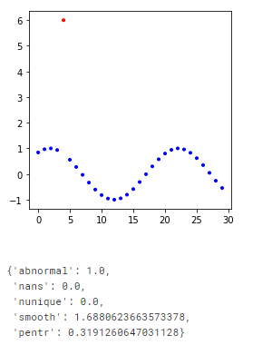
Another point to mention is that it’s useful to add non-informative “noise” features into the set of actual features, and then look into rank position of these noise features to measure the performance of the the feature selection algorithm.

For univariate feature selection we would recommend just using distance correlation (to measure non-linear dependence effects) and pearson correlation (for linear dependence) , as other methods, such as Fisher F-test, Chi2 and tau and spearman correlations would give similar results.

We will use the following python packages:

 pip install xgboost
 pip install logging
 pip install mlextend
 pip install eli5
 pip install pyentrp


The function signature will be the following:

 def runselector(df,y,xs,model,nansy,nansx,methods=None,scoring=None,eval_metric=None,verbose=0,cv=None,eliniter=5,dftest=None):
 

where df is a dataframe (train set)
y is column name for y variable (we predict y ~ xs )
xs is list of feature column names.
nansy = NaN’s substitution rule for y
nansx NaN’s substitution rule for features
methods = list of feature selection methods
scoring = scoring function (i.e. f1)
cv = cross validation iterator
eliniter = number of iterations for eli method
dftest = test dataset (optional)

We will also make this function to work with sklearn’s pipelines, useful when features need scaling, and to avoid information leak from scaling whole dataset.

To run univariate feature selection inside feature selector we will use help function fs1().

def fs1(res,y,xs=None):
    if xs is None:
        xs=res.columns
    xs=list(xs)
    xs=list(set(xs)-set([y]))
    df=res[xs+[y]]
    dcors={}
    pearsons={}
    fctests={}
    frtests={}
    chi2abs={}
    mir={}
    mic={}
    kendalls={}
    for col in xs:
        dfdropna=df[[col,y]].replace([np.inf, -np.inf], np.nan).dropna()
        if dfdropna.shape==(0,2):
            continue
        try:
            fctests[col]=f_classif(dfdropna[[col]],dfdropna[y])[0]
        except:
            pass

        dcors[col]=dcor(dfdropna[col],dfdropna[y])
        pearsons[col]=dfdropna[[col,y]].corr().iloc[1,0]

    corrs=DF(pearsons,index=['pearsonabs']).abs().T.join(DF(dcors,index=['dcor']).T).join(DF(fctests,index=['fc']).T)
    res=pd.concat([corrs,corrs.rank(pct=True).add_prefix('rk.')],axis=1).sort_values(by='rk.dcor',ascending=False) 
    logging.info(f"fs1 rk.dcor index {list(res['rk.dcor'].index)}")
    return res

Example of usage on dummy classification problem with target variable y and features x1,x2,x3 and additional feaature q.x3 (quantile of x3 noise feature) :

from sklearn.ensemble import RandomForestClassifier
import xgboost as xgb
import numpy as np
from dcor import distance_correlation as dcor
from eli5.sklearn import PermutationImportance
from mlxtend.feature_selection import SequentialFeatureSelector
from pyentrp.entropy import permutation_entropy as pentropy
import shap
from scipy.stats import weightedtau as wtau
npa=np.array
DF=pd.DataFrame
import logging

modelxgb=xgb.XGBClassifier(objective ='binary:logistic', colsample_bytree = 1, learning_rate = 1,max_depth = 10, alpha = 1, n_estimators = 5)
x1=npa([-1,-2,-3,-4,-5,6,7,8,9,10,11,12,13,14,15])
np.random.shuffle(x1)
x2=x1+np.random.randn(len(x1))
x3=np.random.randn(len(x1))
y=(x1>0).astype(int)
xs=['x1','x2','x3','q.x3']
dfunittest=DF({'x1':x1,'x2':x2,'x3':x3,'q.x3':pd.qcut(x3,3,labels=False),'y':y})
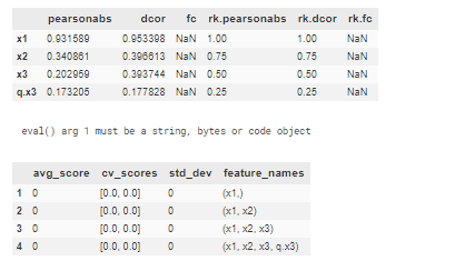
display(fs1(dfunittest,'y',xs))
runselector(dfunittest.iloc[:10],y='y',xs=xs,model=modelxgb,nansy='.fillna(0)',nansx=None,verbose=10,methods=['sfsb','sfsf','eli','shap'],dftest=dfunittest.iloc[-10:],scoring='f1',eval_metric='auc',cv=2)

output:

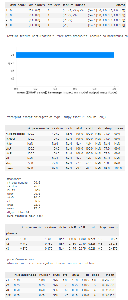
Full code of the feature selection and helper functions:

from sklearn.ensemble import RandomForestClassifier
import xgboost as xgb
import numpy as np
from dcor import distance_correlation as dcor
from eli5.sklearn import PermutationImportance
from mlxtend.feature_selection import SequentialFeatureSelector
from pyentrp.entropy import permutation_entropy as pentropy
import shap
from scipy.stats import weightedtau as wtau
npa=np.array
DF=pd.DataFrame
import logging


def calccorr(df,method='dcor',**kwargs):
    #ipdb.set_trace()
    if method.replace('abs','') in ['pearson','kendall','spearman']:
        dfres=df.corr(method=method.replace('abs','')).rename_axis(method)
        if 'abs' in method:
            return dfres.abs()
        else:
            return dfres
    cols=df.columns
    resd=DF(np.zeros((len(cols),len(cols))),index=cols,columns=cols)
    for icol1 in range(len(cols)):
        for icol2 in range(len(cols)):
            if icol1!=icol2:
                dfdropna=df.iloc[:,[icol1,icol2]].dropna()
                res=eval(method)(dfdropna.iloc[:,0],dfdropna.iloc[:,1],**kwargs)
                if method in ['wtau']:
                    res=res[0]
                if method in ['np.corrcoef']:
                    res=res[1,0]
                resd.iloc[icol1,icol2]=res
            else: #calc pentropy
                #ipdb.set_trace()
                resd.iloc[icol1,icol2]=pentropy(df.iloc[:,[icol1]].dropna().values.flatten(),order=3,delay=1,normalize=True)                
    return resd.rename_axis(method)

pd.core.frame.DataFrame.calccorr=calccorr 


def myround2(ts):
        try:
            return int(np.round(float(ts),2)*100)
        except: pass
        try:
            return (np.round(ts.astype(float),2)*100).astype(int)
        except: pass
        try:
            return {k:(np.round(v,2)*100).astype(int) for k,v in ts.items() }
        except Exception as e:
            pass
        return ts

pd.core.frame.DataFrame.myround2=lambda df:df.applymap(myround2)
pd.core.series.Series.myround2=lambda df:df.apply(myround2)

def fs1(res,y,xs=None):
    if xs is None:
        xs=res.columns
    xs=list(xs)
    xs=list(set(xs)-set([y]))
    df=res[xs+[y]]
    dcors={}
    pearsons={}
    fctests={}
    frtests={}
    chi2abs={}
    mir={}
    mic={}
    kendalls={}
    for col in xs:
        dfdropna=df[[col,y]].replace([np.inf, -np.inf], np.nan).dropna()
        if dfdropna.shape==(0,2):
            continue
        try:
            fctests[col]=f_classif(dfdropna[[col]],dfdropna[y])[0]
        except:
            pass

        dcors[col]=dcor(dfdropna[col],dfdropna[y])
        pearsons[col]=dfdropna[[col,y]].corr().iloc[1,0]

    corrs=DF(pearsons,index=['pearsonabs']).abs().T.join(DF(dcors,index=['dcor']).T).join(DF(fctests,index=['fc']).T)
    res=pd.concat([corrs,corrs.rank(pct=True).add_prefix('rk.')],axis=1).sort_values(by='rk.dcor',ascending=False) 
    logging.info(f"fs1 rk.dcor index {list(res['rk.dcor'].index)}")
    return res

def runselector(df,y,xs,model,nansy,nansx,methods=None,scoring=None,eval_metric=None,verbose=0,cv=None,eliniter=5,dftest=None):
    try:    
        if 'xgb' in model.named_steps['pipe1'].__class__.__name__.lower():
            if eval_metric=='f1':
                eval_metric=minusf1
    except:
        if 'xgb' in 'xgb' in model.__class__.__name__.lower():
            if eval_metric=='f1':
                eval_metric=minusf1
        
    if methods is None:
        methods=['boruta','rfe','sfsb','sfsf','shap','eli']
    
    xs=list(xs)
    if scoring is None:
        if df[y].nunique()<10:
            scoring='balanced_accuracy'
        else:
            scoring='r2'
        print('runselector scoring is None.using {}'.format(scoring))
    
    ytrain=eval('df[y]'+nansy)
    xtrain=eval('df[xs]'+nansx) if nansx is not None else df[xs]
    try:
        inferfreq=pd.infer_freq(df.index)
    except:
        inferfreq=None

    logging.info(f"runselector START df.index.min,max={df.index.min(),df.index.max()} dftest.minmax={dftest.index.min(),dftest.index.max() if dftest is not None else 'None'}  inferfreq={inferfreq} meansecsdiff= {float(np.diff(npa(df.index)).mean())/1e9}secs scoring={scoring} \n modelclass={model.__class__.__name__} modeldict={model.__dict__} xs={xs} \n {df.describe()}")
    
    try:
        model=eval(model)
    except Exception as e:
        print(e)
           
    fs1df=fs1(df,y,xs)
    res=fs1df[fs1df.columns[fs1df.columns.str.contains('rk\\.')]]
    
    if 'boruta' in methods:

        boruta_selector=BorutaPy(model).fit(xtrain,ytrain)#, n_estimators = 10, random_state = 0)
  #      boruta_selector=BorutaPy(model).fit(xtrain.values,ytrain.values)#, n_estimators = 10, random_state = 0)
        boruta=DF({'boruta':boruta_selector.ranking_,'xs':xs}).set_index('xs').rank(ascending=False,pct=True).sort_values(by='boruta',ascending=False)
        logging.info(f'boruta: {boruta.round(2)*100}')
        res=res.join(boruta)
    #boruta_selector = selectormodel
    
    if 'abscoef' in methods:
        try:
#            ipdb.set_trace()
            modelcoef=clone(model)
            modelcoef.fit(xtrain, ytrain)
            rfeselectorranking=np.abs(modelcoef.coef_[0])*xtrain.std() #multiply by feature stddev, ocnditional that feture is centered at 0
            abscoef=DF({'abscoef':rfeselectorranking,'xs':xs}).set_index('xs').rank(ascending=False,pct=True)
            res=res.join(abscoef)
            abscoeflog=DF({'abscoefbystd':rfeselectorranking,'coef':modelcoef.coef_[0],'std':xtrain.std(),'xs':xs}).set_index('xs').sort_values(by='abscoefbystd',ascending=False)
            logging.info(f'abscoef:\n {abscoeflog}')
        except Exception as e:
            print(f"abscoef:{e}")

    if 'rfe' in methods:
        try:
            rfeselector = RFE(model, 1, step=1).fit(xtrain, ytrain)
            rfeselectorranking=rfeselector.ranking_
            rfe=DF({'rfe':rfeselectorranking,'xs':xs}).set_index('xs').rank(ascending=False,pct=True)
            res=res.join(rfe)
        except Exception as e:
            print(f"rfe:{e}")
    if 'sfsf' in methods:
        sfsf = SequentialFeatureSelector(model,k_features=len(xs), forward=True, floating=False,  verbose=0,  scoring=scoring,  cv=cv).fit(xtrain, ytrain,custom_feature_names=xs)
        sfsF=DF(np.unique(DF(sfsf.get_metric_dict()).T['feature_names'].sum(), return_counts=True)).T.set_index(0).rank(pct=True).sort_values(by=1,ascending=False).rename(columns={1:'sfsF'})
        if verbose>1: 
            display(DF(sfsf.get_metric_dict()).T[['avg_score','cv_scores','std_dev','feature_names']])
        res=res.join(sfsF)
        logging.info(f'sfsf:\n {sfsF.round(2)*100}')
    if 'sfsb' in methods:
        sfsb = SequentialFeatureSelector(model,k_features=1, forward=False, floating=False,  verbose=0,  scoring=scoring,  cv=cv).fit(xtrain, ytrain,custom_feature_names=xs)
        sfsB=DF(np.unique(DF(sfsb.get_metric_dict()).T['feature_names'].sum(), return_counts=True)).T.set_index(0).rank(pct=True).sort_values(by=1,ascending=False).rename(columns={1:'sfsB'})

        if verbose>1:
            sfsbd=DF(sfsb.get_metric_dict()).T[['avg_score','cv_scores','std_dev','feature_names']]
            if dftest is not None:
                sfsbd['dftest']=''
                
                for i,row in sfsbd.iterrows():
                    if 'Pipe' in model.__class__.__name__:
                        model.fit(df[list(row['feature_names'])],df[y],pipe1__eval_metric=eval_metric,pipe1__eval_set=[(dftest[list(row['feature_names'])], dftest[y])],pipe1__verbose=0)
                        sfsbd.at[i,'dftest'] = model.named_steps['pipe1'].evals_result()['validation_0']
                    else:
                        model.fit(df[list(row['feature_names'])],df[y],eval_metric=eval_metric,eval_set=[(dftest[list(row['feature_names'])], dftest[y])],verbose=0)
                        sfsbd.at[i,'dftest'] = model.evals_result()['validation_0']
                    
                    print(list(row['feature_names']),eval_metric,sfsbd.at[i,'dftest'])
            logging.info(f"sfsbd=\n{sfsbd.myround2()}")
            display(sfsbd.round(3))
        logging.info(f'sfsb:\n {sfsB.round(2)*100}')
        res=res.join(sfsB)
        
    model.fit(xtrain,ytrain)
    
    if 'eli' in methods:
        if cv is None:
            cv='prefit'
        permuter = PermutationImportance(model, scoring=None, cv=cv, n_iter=eliniter, random_state=42)#instantiate permuter object #'balanced_accuracy'  'prefit'
        elidf=DF({'eli':permuter.fit(xtrain.values,ytrain.values).feature_importances_,'xs':xs}).set_index('xs').rank(ascending=True,pct=True).sort_values(by='eli',ascending=False)
        logging.info(f'eli: {elidf.round(2)*100}')
        res=res.join(elidf)
            
    if 'shap' in methods:
        if 'Pipe' in model.__class__.__name__:
            if 'xgb' in model.named_steps['pipe1'].__class__.__name__.lower() and model.named_steps['pipe1'].get_params()['booster'] in ('gbtree',None):
                explainer=shap.TreeExplainer(model.named_steps['pipe1'],model_output='raw')
            elif 'NN' in model.named_steps['pipe1'].__class__.__name__:
                explainer=shap.DeepExplainer(model.named_steps['pipe1'].model.model, data=xtrain.values)#, session=None, learning_phase_flags=None)
            elif 'Logistic' in model.named_steps['pipe1'].__class__.__name__:
                explainer=shap.KernelExplainer(model.named_steps['pipe1'].predict_proba, data=xtrain.values, link='logit',l1_reg='aic')
            else:
                raise ValueError(f"shap for model {model.named_steps['pipe1'].__class__.__name__} {model.named_steps['pipe1'].get_params()} not imlemented in fs.py")
        else:
            if 'xgb' in model.__class__.__name__.lower() and model.get_params()['booster'] in ('gbtree',None):
                explainer=shap.TreeExplainer(model,model_output='raw')
            elif 'NN' in model.__class__.__name__:
                explainer=shap.DeepExplainer(model.model.model, data=xtrain.values)#, session=None, learning_phase_flags=None)
            elif 'Logistic' in model.__class__.__name__:
                explainer=shap.KernelExplainer(model.predict_proba, data=xtrain.values, link='logit',l1_reg='aic')
            else:
                raise ValueError(f"shap for model {model.__class__.__name__} and params={model.get_params()} not imlemented in fs.py")

        try:

            shap_values = explainer.shap_values(xtrain.values)#, tree_limit=5)
            concat=np.concatenate(shap_values) if type(shap_values)==type([]) else shap_values
            shap_abs = np.abs(concat)
            global_importances = np.nanmean(shap_abs, axis=0)
            indices = np.argsort(global_importances)[::-1]
            features_ranked = []
            for f in range(df[xs].shape[1]):
                features_ranked.append(xs[indices[f]])
            shapdf=DF({'shap':global_importances},index=xs).rank(ascending=True,pct=True)
            res=res.join(shapdf)
            if verbose>2:
                shap.summary_plot(shap_values, df[xs], plot_type="bar",class_names=model.classes_)
                shap.initjs()
                try:
                    for i in range(len(explainer.expected_value)):
                        display(shap.force_plot(explainer.expected_value[i], shap_values[i],df[xs]))
                except Exception as e:
                    print(f"forceplot exception:{e}")
        except Exception as e:
            logging.warning(f"shaps exception = {e}")            
            
    res['mean']=res.mean(axis=1)
    res=res.sort_values(by='mean',ascending=False)
    
    if verbose>1:
        logging.info(f"res.corr.mean=\n{100*res.corr().round(2)}")
        display(100*res.corr().round(2))
        print(f"meancorr=\n{res.corr().mean().round(2)*100}")
        logging.info(f"meancorr=\n{res.corr().mean().myround2()}")
        
    if verbose>1:
        res1=res.copy()
        res1['pfname']=res1.index.str.split('.').str[-1]
        res1=res1.groupby('pfname').mean().sort_values(by='mean',ascending=False)#.set_index('pfname')
        print("pure features mean rank")
        display(res1)
        logging.info(f"pure fs mean rank\n {res1.myround2()}")
        print("pure features wtau")
        try:
            display(100*res1.calccorr(method='wtau').round(2))
            logging.info(f"pure features wtau \n{res1.calccorr(method='wtau').myround2()}")
        except Exception as e:
            print(f"wtau calcorr exception{str(e)}")
     
    logging.info(f"runselector complete res=\n{res.round(2)*100} {list(res.index)}")
    return res

To run the feature selection on the scaled features one can use the same function and pipe as following:


model=Pipeline([("pipe0",StandardScaler()),("pipe1",xgb.XGBClassifier(objective ='binary:logistic', colsample_bytree = 1, learning_rate = 1,max_depth = 10, alpha = 1, n_estimators = 5))])

Posted in machine learning Tagged with: ,

How to display candle stick bars from binance futures in jupyter notebook

In order to download and display binance candlestick bars in jupyter notebook we will need the following packages:

pip install mplfinance
pip install python-binance
pip install plotly

Also you would need to get API keys from binance Binance API management .

We will download and display two candle stick charts for ETH futures, one using mplfinance library, and another using plotly.
We will use 1 minute ETHUSDT futures data.

from binance.client import Client

from plotly.offline import download_plotlyjs, init_notebook_mode, plot, iplot
import cufflinks as cf
cf.go_offline()
init_notebook_mode(connected=True)

import pandas as pd
import datetime as dt
import matplotlib.pyplot as plt
%matplotlib inline
from dateutil import parser
import math
import os.path
import time
import plotly.graph_objects as go
from datetime import datetime
import mplfinance as mpf

binance_api_key = '<YOUR API KEY>'
binance_api_secret = '<YOUR API SECRET>'

binsizes = {"1m": 1, "5m": 5, "1h": 60, "1d": 1440}
batch_size = 750
binance = Client(api_key=binance_api_key, api_secret=binance_api_secret,)

def binanceklines(symbol='ETHUSDT',interval='1m',limit=500,since="1 day ago UTC"):
    klines = binance.futures_klines(symbol='ETHUSDT',interval={'1m':Client.KLINE_INTERVAL_1MINUTE,'5m':Client.KLINE_INTERVAL_5MINUTE}[interval],since=since,limit=limit)
    data = pd.DataFrame(klines, columns = ['ts', 'o', 'h', 'l', 'c', 'v', 'close_time', 'quote_av', 'trades', 'tb_base_av', 'tb_quote_av', 'ignore' ])
    data=data.apply(pd.to_numeric)
    data['ts'] = pd.to_datetime(data['ts'], unit='ms')
    data=data.set_index('ts')
    return data

df=binanceklines(limit=None)
fig = go.Figure(data=[go.Candlestick(x=df.index,open=df['o'],high=df['h'],low=df['l'],close=df['c'])])
fig.show()

plt.rcParams["figure.figsize"] = (10,8)
mpf.plot(df.rename(columns={'o':'Open','h':'High','l':'Low','c':'Close','v':'Volume'}).apply(pd.to_numeric),type='bars',volume=True,mav=(20,40),figscale=3,style='charles')

This results in:

The advantage of plotly chart is that it’s more interactive.

In case your are interested to 10% binance promo code discount on binance trading fees, you can use the following code: WFH7DYED

Posted in crypto Tagged with: , ,

How to check time-series for abnormality

In many time series machine learning problems the with large number of features the raw data might contain

– abnormal / extreme points
– discontinuities
– stale data

To help with determining quickly abnormal or extreme points we can use z-transform of the time series.
To dtermine if time series contain discountinuities we can calculate how much removing one point changes sum of first difference of the time series.
and lastly to determine stale/predictable data we can use permutation-entropy implemented in python package pyentrp.

The code to run all the 3 tests at once is present below:

from scipy.stats import chi2 
from pyentrp.entropy import permutation_entropy as pentropy

def smoothcoef(y):
    y=npa(y).flatten()
    ymax=max(np.abs(y).max(),0.0000001)
    tv=np.zeros(len(y))
    for i in range(len(y)-1):
        try:
            tv[i]=np.abs(np.diff(np.delete(y,i),1)).sum()
        except:
            ipdb.set_trace()
    tv=np.delete(tv,[0,len(tv)-1])
    tv=np.abs(np.diff(tv,1))
    return tv.max()/ymax

def abnormality(ts,thresh,retpoints=False,plot=False): #high values means abnormal
        avg=ts.mean()
        var=ts.var()
        nans=ts.isnull().sum()/len(ts)
        abnormal=(ts-avg)**2/var >chi2.interval(1-thresh, 1)[1]
        if plot:
            if (plot=='abnormal' and abnormal.any()) or plot=='all':                
                plt.figure(figsize = (4, 4))
                plt.clf()
                plt.scatter(ts.index,ts.values,c=abnormal,cmap='bwr',marker='.') 
                plt.show()
        res={}
        if retpoints:
            res['abnpoints']=ts[abnormal]
        return {**res,'abnormal':float(abnormal.any()),'nans':nans,'nunique':1-ts.nunique()/len(ts),'smooth':smoothcoef(ts.dropna()),'pentr':1-pentropy(ts.dropna(),normalize=True)}

Example usage is shown in the following code:

DF=pd.DataFrame
df=DF({'x':np.linspace(1,10,30)})
df['y']=np.sin(df['x'])
df
df['y'].iloc[4]=6
df[['y']].plot()
abnormality(df['y'],0.001,retpoints=False,plot='abnormal')

the result is show on the following figure:

Interpretation of the results is the following:

Higher the number => more probability there is abnormality in the time series.
When plot parameter is specified graph will be shown with abnormal points in red.

Posted in machine learning Tagged with: ,