Here we’ll show an example of code for CVA calculation (credit valuation adjustment) using python and Quantlib with simple Monte-Carlo method with portfolio consisting just of a single interest rate swap.It’s easy to generalize code to include more financial instruments , supported by QuantLib python Swig interface.
CVA calculation algorithm:
1) Simulate yield curve at future dates
2) Calculate your derivatives portfolio NPV (net present value) at each time point for each scenario
3) Calculate CVA as sum of Expected Exposure multiplied by probability of default at this interval
$$ CVA = (1-R) \int{DF(t) EE(t) dQ_t} $$
where R is Recovery (normally set to 40%) EE(t) expected exposure at time t and dQ survival probability density , DF(t) discount factor at time t
Outline
1) In this simple example we will use Hull White model to generate future yield curves. In practice many banks use some yield curve evolution models based on historical simulations.
In Hull White model short rate $$ r_t $$ is distributed normally with known mean and variance.
2) For each point of time we will generate whole yield curve based on short rate. Then we will price our interest rate swap on each of these curves.
after
3) to approximate CVA we will use BASEL III formula for regulatory capital charge approximating default probability [or survival probability ] as exp(-ST/(1-R))
so we get
$$ CVA= (1-R) \sum \frac{EE^{*}_{T_{i}}+EE^{*}_{T_{i-1}}}{2} (e^{-\frac{ST_{i-1}}{1-R}}-e^{-\frac{ST_{i}}{1-R}})^+ $$
where $$ EE^{*} $$ is discounted Expected exposure of portfolio
Details
For this first example we’ll take 5% flat forward yield curve. In the second test example below we’ll take full curve as of 26/12/2013.
1) Hull-White model for future yield curve simulations
the model is given by dynamics:
$$ dr_t=(\theta_t-ar_t)dt+\sigma dW_t $$
We will use that in Hull White model short rate $$ r_t $$ is distributed normally with mean and variance given by
$$ E(r_t|r_s)=r_se^{-a(t-s)}+\gamma_t-\gamma_se^{-a(t-s)}$$
$$ Var(r_t|r_s)=\frac{\sigma^2}{2a}(1-e^{-2a(t-s)})$$
where $$ \gamma_t=f_t(0)+\frac{\sigma^2}{2a}(1-e^{-at})^2 $$
and $$ f_t(0) $$ is instantaneous forward rate at time t as seen at time 0.
The calculations will not depend on $$\theta_t$$.
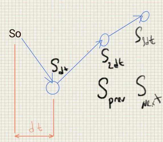
To generate future values of $$ r_t $$ first we will generate matrix of standard normal variables using numpy library function numpy.random.standard_normal().After that we will apply transform $$ mean+\sqrt{variance} Normal(0,1) $$ to get $$ r_t $$
after getting matrix of all $$ r_t $$ for all simulations and time points we will construct yield curve for each $$ r_t $$ using Hull White discount factors $$ P_{->T}(t)=A(t,T)e^{-B(t,T)r_t} $$ for 20 years and store each yield curve in matrix crvMat
2) Valuing portfolio
On each of this curve we will value swap using QuantLib function. you can add more financial instruments just by adding its value to global NPV
For our exzample portfolio we’ll take one interest rate swap EUR 10MM notional receiving 5% every 6m , TARGET calendar, with 5 years maturity.
Actual/360 daycounter for both legs.
3) CVA calculation
After getting matrix of all NPV at each point for each simulation we will replace negative values with 0.
Then we average each column of the matrix (corresponding to averaging for each time point) to get Expected Exposure.
and finally calculate CVA as sum as in BASEL 3 formula.
here we’ll take 500bps flat CDS spread.
Python Code for CVA calculation
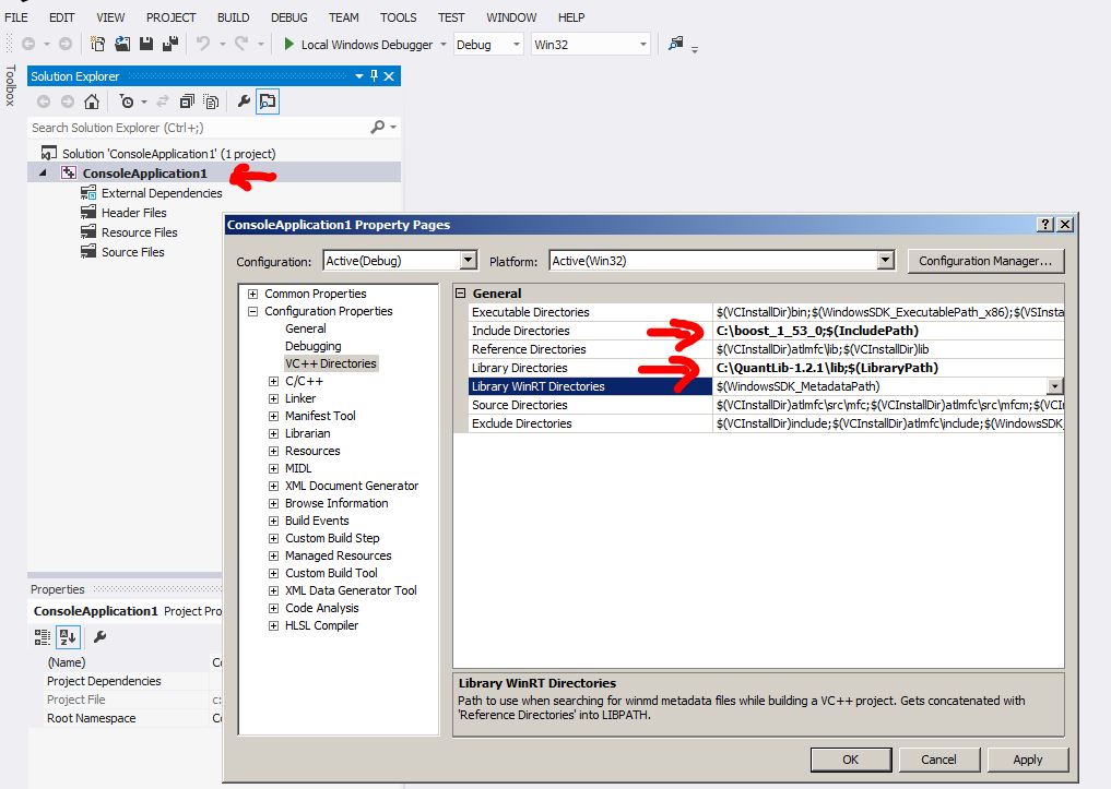
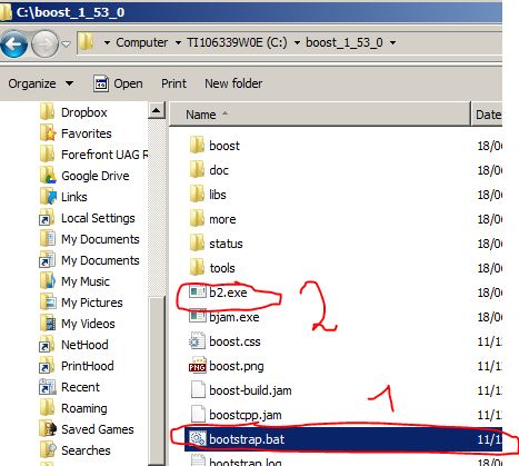
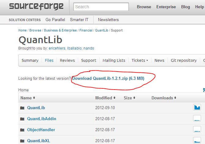
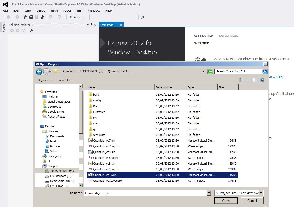
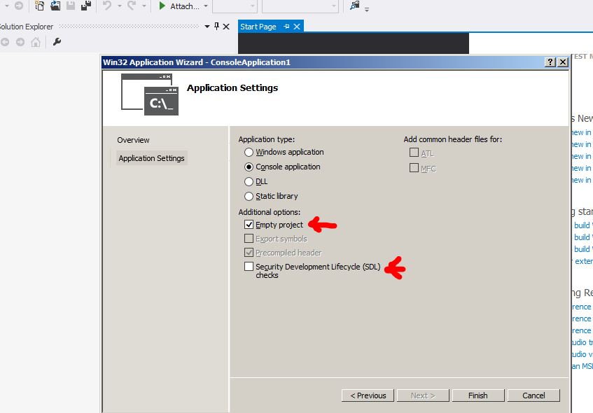
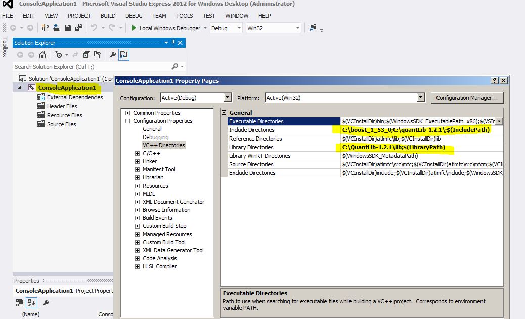
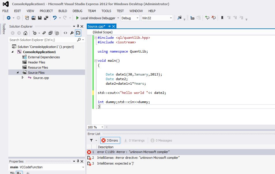
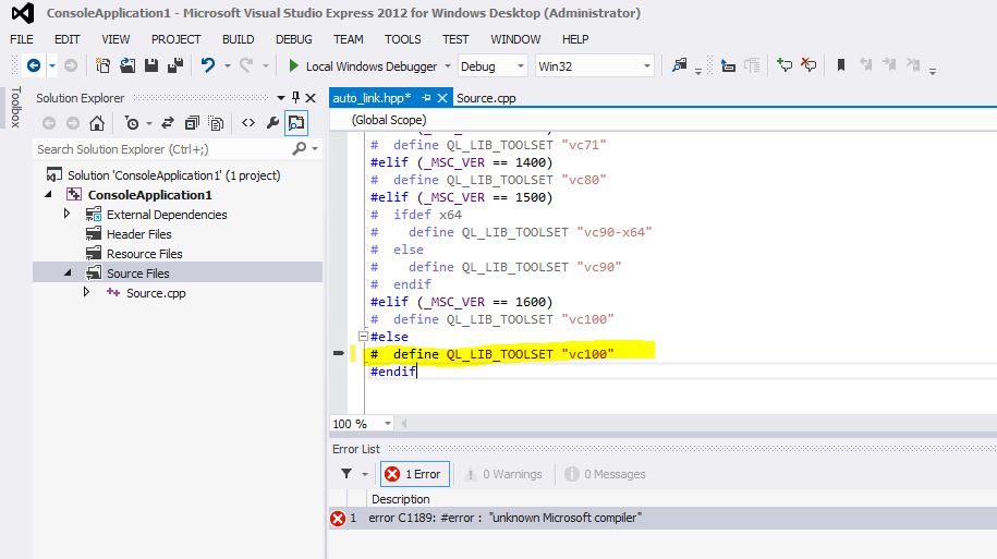
First , Install QuantLib package for python (use guide here )
to run the program just copy paste it into iPython editor and press enter
#(c) 2013 PriceDerivatives.com
# Distributed without any warranty.For educational purposes only.

from  QuantLib import *
import numpy as np
from math import *
from pylab import *

def A(t,T):
    forward = crvToday.forwardRate(t, t,Continuous, NoFrequency).rate()
    value = B(t,T)*forward - 0.25*sigma*B(t,T)*sigma*B(t,T)*B(0.0,2.0*t);
    return exp(value)*crvToday.discount(T)/crvToday.discount(t);

def B(t,T):
    return (1.0-exp(-a*(T-t)))/a;

def gamma(t):
        forwardRate =crvToday.forwardRate(t, t, Continuous, NoFrequency).rate()
        temp = sigma*(1.0 - exp(-a*t))/a
        return (forwardRate + 0.5*temp*temp)

def gamma_v(t):
    res=np.zeros(len(t))
    for i in xrange(len(t)):
        res[i]=gamma(t[i])
    return res

Nsim=100
a=0.1
sigma=0.02

todaysDate=Date(30,12,2013);
Settings.instance().evaluationDate=todaysDate;
crvToday=FlatForward(todaysDate,0.02,Actual360())

r0=forwardRate =crvToday.forwardRate(0,0, Continuous, NoFrequency).rate()
months=range(1,12*5,1)
sPeriods=[str(month)+"m" for month in months]
Dates=[todaysDate]+[todaysDate+Period(s) for s in sPeriods]
T=[0]+[Actual360().yearFraction(todaysDate,Dates[i]) for i in xrange(1,len(Dates))]
T=np.array(T)
rmean=r0*np.exp(-a*T)+ gamma_v(T) -gamma(0)*np.exp(-a*T)

np.random.seed(1)
stdnorm = np.random.standard_normal(size=(Nsim,len(T)-1))

rmat=np.zeros(shape=(Nsim,len(T)))
rmat[:,0]=r0

for iSim in xrange(Nsim):
    for iT in xrange(1,len(T)):
        mean=rmat[iSim,iT-1]*exp(-a*(T[iT]-T[iT-1]))+gamma(T[iT])-gamma(T[iT-1])*exp(-a*(T[iT]-T[iT-1]))
        var=0.5*sigma*sigma/a*(1-exp(-2*a*(T[iT]-T[iT-1])))
        rmat[iSim,iT]=mean+stdnorm[iSim,iT-1]*sqrt(var)

startDate=Date(30,12,2013);

crvMat= [ [ 0 for i in xrange(len(T)) ] for iSim in range(Nsim) ]
npvMat= [ [ 0 for i in xrange(len(T)) ] for iSim in range(Nsim) ]

for row in crvMat:
    row[0]=crvToday

for iT in xrange(1,len(T)):
    for iSim in xrange(Nsim):
        crvDate=Dates[iT];
        crvDates=[crvDate]+[crvDate+Period(k,Years) for k in xrange(1,21)]
        crvDiscounts=[1.0]+[A(T[iT],T[iT]+k)*exp(-B(T[iT],T[iT]+k)*rmat[iSim,iT]) for k in xrange(1,21)]
        crvMat[iSim][iT]=DiscountCurve(crvDates,crvDiscounts,Actual360(),TARGET())

#indexes definitions
forecastTermStructure = RelinkableYieldTermStructureHandle()
index = Euribor(Period("6m"),forecastTermStructure)

#swap 1 definition
maturity = Date(30,12,2018);
fixedSchedule = Schedule(startDate, maturity,Period("6m"), TARGET(),ModifiedFollowing,ModifiedFollowing,DateGeneration.Forward, False)
floatingSchedule = Schedule(startDate, maturity,Period("6m"),TARGET() ,ModifiedFollowing,ModifiedFollowing,DateGeneration.Forward, False)
swap1 = VanillaSwap(VanillaSwap.Receiver, 1000000,fixedSchedule,0.05 , Actual360(),floatingSchedule, index, 0,Actual360())  #0.01215

for iT in xrange(len(T)):
    Settings.instance().evaluationDate=Dates[iT]
    allDates= list(floatingSchedule)
    fixingdates=[index.fixingDate(floatingSchedule[iDate]) for iDate in xrange(len(allDates)) if index.fixingDate(floatingSchedule[iDate])<=Dates[iT]]
    if fixingdates:
        for date in fixingdates[:-1]:
            try:index.addFixing(date,0.0)
            except:pass
        try:index.addFixing(fixingdates[-1],rmean[iT])
        except:pass
    discountTermStructure = RelinkableYieldTermStructureHandle()
    swapEngine = DiscountingSwapEngine(discountTermStructure)
    swap1.setPricingEngine(swapEngine)

    for iSim in xrange(Nsim):
        crv=crvMat[iSim][iT]
        discountTermStructure.linkTo(crv)
        forecastTermStructure.linkTo(crv)
        npvMat[iSim][iT]=swap1.NPV()

npvMat=np.array(npvMat)
npvMat[npvMat<0]=0
EE=np.mean(npvMat,axis=0)

S=0.05 #constant CDS spread
R=0.4  #Recovery rate 40%

sum=0
#calculate CVA
for i in xrange(len(T)-1):
    sum=sum+0.5*(EE[i]*crvToday.discount(T[i])+EE[i+1]*crvToday.discount(T[i+1]))*(exp(-S*T[i]/(1.0-R))-exp(-S*T[i+1]/(1.0-R)))
CVA=(1.0-R)*sum

print "\nCVA=",CVA

plot(T,EE)
print "\nEE\n",npvMat
show()
Output
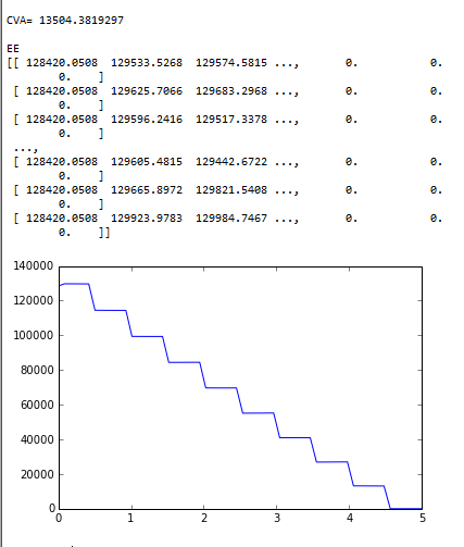
CVA expected exposure swap
for simple current net exposure method see Current Net Exposure excel example
Tests with 2% swap
For test results lets take 2% EUR 10MM notional interest rate receiver swap with semiannual payments fixed and floating leg.
To check validity of the python code we can check several quantities:
$$ E(r_{t_i}) $$ for each future date
$$ P_{\rightarrow T}(0)= E( e^{-\int_0^Tr_sds})=E( E(e^{-\int_0^Tr_sds}|F_{t_i}))=E(P_{\rightarrow t_i}(0)E(e^{-\int_{t_i}^Tr_sds}|F_{t_i})) $$ for each future time point $$ t_i $$ $$T is maturity $$
also we'll output some generated yield curves.
from QuantLib import *
import numpy as np
from math import *
from pylab import *
def A(t,T):
evaldate=Settings.instance().evaluationDate
forward = crvToday.forwardRate(t, t,Continuous, NoFrequency).rate()
value = B(t,T)*forward - 0.25*sigma*B(t,T)*sigma*B(t,T)*B(0.0,2.0*t);
return exp(value)*crvToday.discount(T)/crvToday.discount(t);
def B(t,T):
return (1.0-exp(-a*(T-t)))/a;
def gamma(t):
forwardRate =crvToday.forwardRate(t, t, Continuous, NoFrequency).rate()
temp = sigma*(1.0 - exp(-a*t))/a
return (forwardRate + 0.5*temp*temp)
def gamma_v(t): #vectorized version of gamma(t)
res=np.zeros(len(t))
for i in xrange(len(t)):
res[i]=gamma(t[i])
return res
Nsim=1000
#a=0.03
#sigma=0.00743
#parameters calibrated with Quantlib to coterminal swaptions on 26/dec/2013
a=0.376739
sigma=0.0209835
todaysDate=Date(26,12,2013);
Settings.instance().evaluationDate=todaysDate;
crvTodaydates=[Date(26,12,2013),
Date(30,6,2014),
Date(30,7,2014),
Date(29,8,2014),
Date(30,9,2014),
Date(30,10,2014),
Date(28,11,2014),
Date(30,12,2014),
Date(30,1,2015),
Date(27,2,2015),
Date(30,3,2015),
Date(30,4,2015),
Date(29,5,2015),
Date(30,6,2015),
Date(30,12,2015),
Date(30,12,2016),
Date(29,12,2017),
Date(31,12,2018),
Date(30,12,2019),
Date(30,12,2020),
Date(30,12,2021),
Date(30,12,2022),
Date(29,12,2023),
Date(30,12,2024),
Date(30,12,2025),
Date(29,12,2028),
Date(30,12,2033),
Date(30,12,2038),
Date(30,12,2043),
Date(30,12,2048),
Date(30,12,2053),
Date(30,12,2058),
Date(31,12,2063)]
crvTodaydf=[1.0,
0.998022,
0.99771,
0.99739,
0.997017,
0.996671,
0.996337,
0.995921,
0.995522,
0.995157,
0.994706,
0.994248,
0.993805,
0.993285,
0.989614,
0.978541,
0.961973,
0.940868,
0.916831,
0.890805,
0.863413,
0.834987,
0.807111,
0.778332,
0.750525,
0.674707,
0.575192,
0.501258,
0.44131,
0.384733,
0.340425,
0.294694,
0.260792
]
crvToday=DiscountCurve(crvTodaydates,crvTodaydf,Actual360(),TARGET())
#crvToday=FlatForward(todaysDate,0.0121,Actual360())
r0=forwardRate =crvToday.forwardRate(0,0, Continuous, NoFrequency).rate()
months=range(3,12*5+1,3)
sPeriods=[str(month)+"m" for month in months]
print sPeriods
Dates=[todaysDate]+[todaysDate+Period(s) for s in sPeriods]
T=[0]+[Actual360().yearFraction(todaysDate,Dates[i]) for i in xrange(1,len(Dates))]
T=np.array(T)
rmean=r0*np.exp(-a*T)+ gamma_v(T) -gamma(0)*np.exp(-a*T)
rvar=sigma*sigma/2.0/a*(1.0-np.exp(-2.0*a*T))
rstd=np.sqrt(rvar)
np.random.seed(1)
stdnorm = np.random.standard_normal(size=(Nsim,len(T)-1))
rmat=np.zeros(shape=(Nsim,len(T)))
rmat[:,0]=r0
for iSim in xrange(Nsim):
for iT in xrange(1,len(T)):
mean=rmat[iSim,iT-1]*exp(-a*(T[iT]-T[iT-1]))+gamma(T[iT])-gamma(T[iT-1])*exp(-a*(T[iT]-T[iT-1]))
var=0.5*sigma*sigma/a*(1-exp(-2*a*(T[iT]-T[iT-1])))
rnew=mean+stdnorm[iSim,iT-1]*sqrt(var)
#if (rnew<0): rnew=0.001
rmat[iSim,iT]=rnew
bonds=np.zeros(shape=rmat.shape)
#E(E(exp(rt)|ti) test
for iSim in xrange(Nsim):
for iT in xrange(1,len(T)):
bonds[iSim,iT]=bonds[iSim,iT-1]+rmat[iSim,iT]*(T[iT]-T[iT-1])
bonds=-bonds;
bonds=np.exp(bonds)
bondsmean=np.mean(bonds,axis=0)
#plot(T,bondsmean)
#plot(T,[crvToday.discount(T[iT]) for iT in xrange(len(T))])
#show()
startDate=Date(26,12,2013);
crvMat= [ [ 0 for i in xrange(len(T)) ] for iSim in range(Nsim) ]
npvMat= [ [ 0 for i in xrange(len(T)) ] for iSim in range(Nsim) ]
for row in crvMat:
row[0]=crvToday
for iT in xrange(1,len(T)):
for iSim in xrange(Nsim):
crvDate=Dates[iT];
crvDates=[crvDate]+[crvDate+Period(k,Years) for k in xrange(1,21)]
rt=rmat[iSim,iT]
#if (rt<0): rt=0
crvDiscounts=[1.0]+[A(T[iT],T[iT]+k)*exp(-B(T[iT],T[iT]+k)*rt) for k in xrange(1,21)]
crvMat[iSim][iT]=DiscountCurve(crvDates,crvDiscounts,Actual360(),TARGET())
bondT=np.zeros(shape=rmat.shape)
for iSim in xrange(Nsim):
for iT in xrange(len(T)):
bondT[iSim,iT]=bonds[iSim,iT]*crvMat[iSim][iT].discount(19-T[iT])
bondTmean=np.mean(bondT,axis=0)
np.set_printoptions(precision=4,suppress=True)
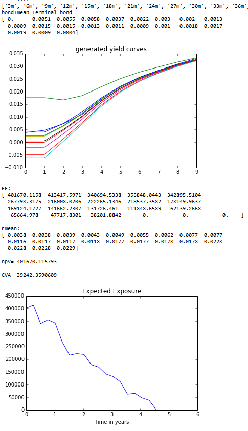
print 'bondTmean-Terminal bond\n',bondTmean-crvToday.discount(19)
plot(range(10),[crvMat[0][0].forwardRate(k, k,Continuous, NoFrequency).rate() for k in range(10)])
for i in xrange(min(Nsim,10)):
plot(range(10),[crvMat[i][1].forwardRate(k, k,Continuous, NoFrequency).rate() for k in range(10)])
title('generated yield curves')
show()
#indexes definitions
forecastTermStructure = RelinkableYieldTermStructureHandle()
index = Euribor(Period("6m"),forecastTermStructure)
#swap 1 definition
maturity = Date(26,12,2018);
fixedSchedule = Schedule(startDate, maturity,Period("6m"), TARGET(),ModifiedFollowing,ModifiedFollowing,DateGeneration.Forward, False)
floatingSchedule = Schedule(startDate, maturity,Period("6m"),TARGET() ,ModifiedFollowing,ModifiedFollowing,DateGeneration.Forward, False)
swap1 = VanillaSwap(VanillaSwap.Receiver, 10000000,fixedSchedule,0.02, Actual360(),floatingSchedule, index, 0,Actual360()) #0.01215
for iT in xrange(len(T)):
Settings.instance().evaluationDate=Dates[iT]
allDates= list(floatingSchedule)
fixingdates=[index.fixingDate(floatingSchedule[iDate]) for iDate in xrange(len(allDates)) if index.fixingDate(floatingSchedule[iDate])<=Dates[iT]]
if fixingdates:
for date in fixingdates[:-1]:
try:index.addFixing(date,0.0)
except:pass
try:index.addFixing(fixingdates[-1],rmean[iT])
except:pass
discountTermStructure = RelinkableYieldTermStructureHandle()
swapEngine = DiscountingSwapEngine(discountTermStructure)
swap1.setPricingEngine(swapEngine)
for iSim in xrange(Nsim):
crv=crvMat[iSim][iT]
discountTermStructure.linkTo(crv)
forecastTermStructure.linkTo(crv)
npvMat[iSim][iT]=swap1.NPV()
npvMat=np.array(npvMat)
npv=npvMat[0,0]
#replace negative values with 0
npvMat[npvMat<0]=0
EE=np.mean(npvMat,axis=0)
print '\nEE:\n',EE
#print '\nrmat:\n',rmat
print '\nrmean:\n',rmean
#print '\nrstd:\n',rstd
#print '\n95% are in \n',zip(rmean-2*rstd,rmean+2*rstd)
S=0.05
R=0.4
sum=0
for i in xrange(len(T)-1):
sum=sum+0.5*crvToday.discount(T[i+1])*(EE[i]+EE[i+1])*(exp(-S*T[i]/(1.0-R))-exp(-S*T[i+1]/(1.0-R)))
CVA=(1.0-R)*sum
print "\nnpv=",npv
print "\nCVA=",CVA
plot(T,EE)
title('Expected Exposure')
xlabel('Time in years')
#plot(T,np.mean(rmat,axis=0))
#plot(T,rmean)
#plot(T,[npvMat[0,0]]*len(T))
show()
print "\nnpv",npvMat
output:
credit value adjustment
Expected exposure
bloomberg CVA = 35266
NB: bloomberg's Exposure is our exposure multiplied by (1-R)
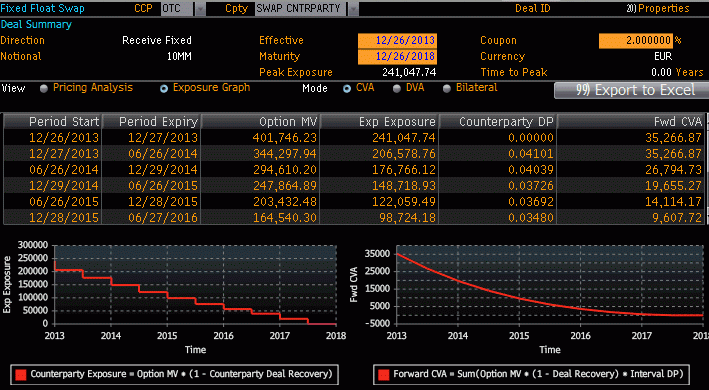
CVA swap