Here we will present simple python code of delta hedging example of a call option .
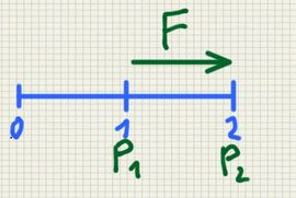
it’s a minimal example with zero interest rates , no dividends. On day 1 we sell 10 near ATM call options and start delta hedging i.e. buying/selling stock so that change in stock price neutralizes change in options value.The portfolio is then $$\pi= delta*Stock-callOption+cashAccount$$
to simulate stock prices we will use log-normal dynamics $$ \frac{dS_t}{S_t} =\sigma_t dW_t $$
We will also simulate implied volatility as log-normal $$ \frac{d\sigma_t}{\sigma_t}=\xi dB_t $$
each day of simulation we will store in DataFrame df , so it will be easy to print and plot with pandas library.
to run the python code you will need pandas library installed in your distribution
apart from usual NPV of hedging portfolio and values of call option and greeks we will also display P&L prediction which is $$ PNL \approx \frac{\Gamma}{2} (dS)^2 + \theta dt $$
delta hedging simulation
first 10 days of delta hedging:
       spot   vol  shares      cash  option   npv    vega  gamma  theta  pnlPredict   pnl  error
0    100.00 30.00    0.00      0.00    0.00  0.00    0.00   0.00   0.00        0.00   nan    nan
1    102.89 29.83    6.35   -401.20  252.38  0.00 -772.52  -0.06   0.12       -0.14  0.00   0.00
2    103.65 29.89    6.40   -406.13  257.56 -0.36 -774.36  -0.06   0.12        0.10 -0.36  -0.46
3     98.00 29.34    6.02   -368.79  218.14  2.91 -754.75  -0.07   0.11       -0.96  3.27   4.23
4     96.83 29.61    5.95   -362.24  213.06  0.93 -748.61  -0.07   0.11        0.06 -1.98  -2.04
5     95.76 29.35    5.86   -353.97  204.68  2.96 -743.77  -0.07   0.11        0.07  2.03   1.96
6     95.40 28.75    5.81   -348.68  198.03  7.53 -742.86  -0.07   0.11        0.10  4.57   4.46
7     94.12 28.71    5.71   -339.71  190.26  7.85 -735.94  -0.07   0.11        0.05  0.32   0.28
8     94.28 27.96    5.69   -336.97  185.56 13.47 -737.79  -0.07   0.10        0.10  5.62   5.52
9     95.42 27.56    5.75   -343.04  189.00 16.52 -744.17  -0.07   0.10        0.05  3.05   3.00
10    96.53 28.02    5.85   -353.01  198.72 13.16 -748.41  -0.07   0.11        0.06 -3.36  -3.42
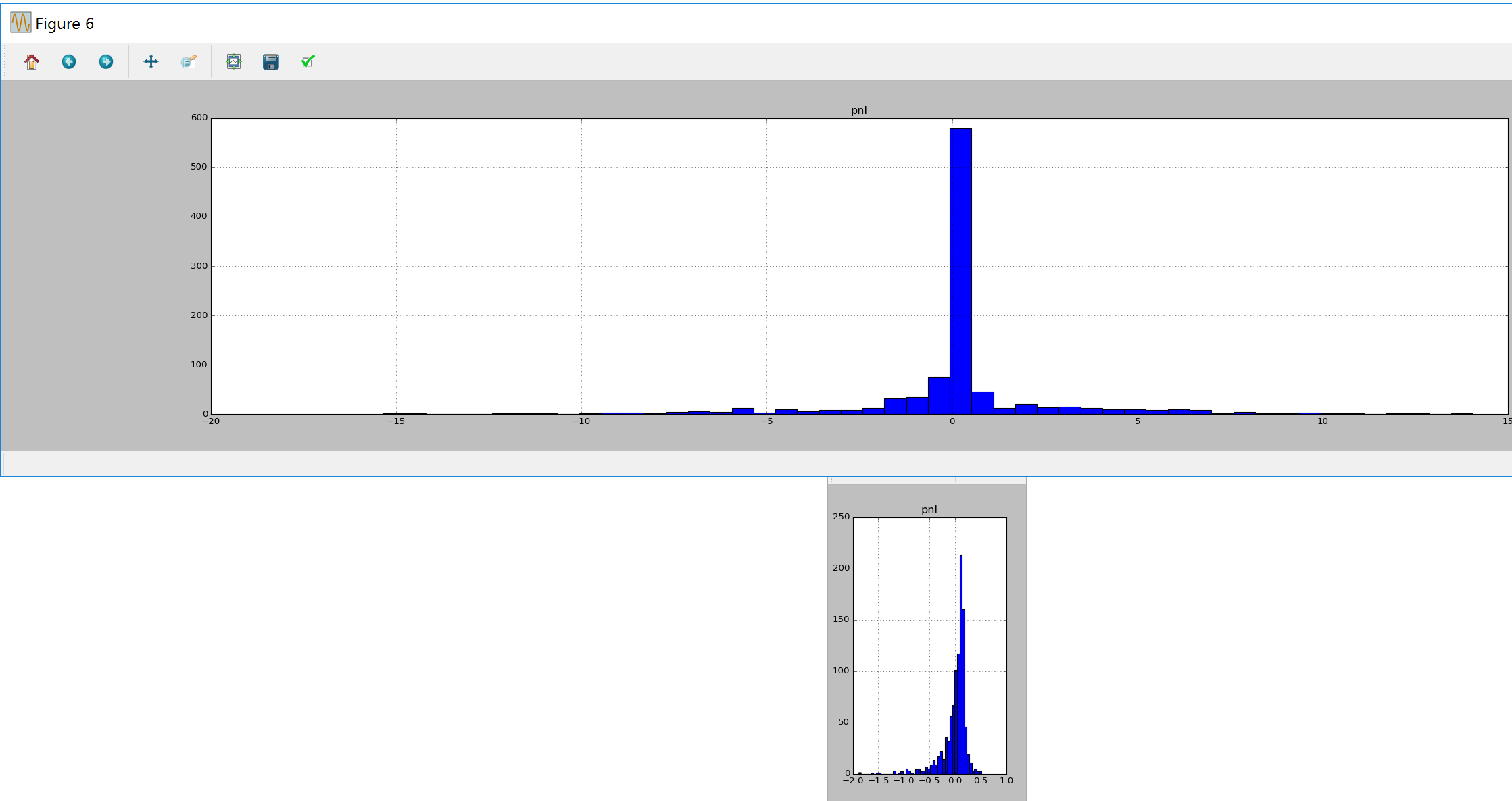
P&L profile
running this code for number of days 10,100,1000,10000 we can see P&L profile start to look narrower and more centered at 0 with number of days , in the limit of infinite days (equivalent to infinite frequency of hedging of Black Scholes assumptions) it would look like a dirac function.
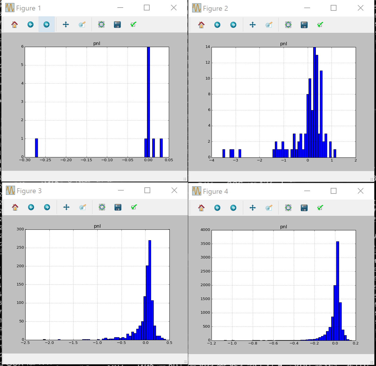
pnl profile delta hedging 10 100 1000 10000 days
Why is it skewed to the left? as Gamma is always negative and high near ATM, if there’s jump down, PNL is proportional to gamma * jump size $$ PNL \approx \frac{\Gamma S^2}{2}((\frac{dS}{S})^2-\sigma^2)$$ and delta makes a high decrease, so we would need to sell many shares cheap. In case there’s a jump up, we would still need to buy more stock (as delta of call option goes up), so still would loose money in this case.That makes the daily PNL profile asymmetric.
Theta
setting Spot prices constant in the code we can see the Theta effect on the hedging strategy:
here’s the example of running the python code with constant Spot:
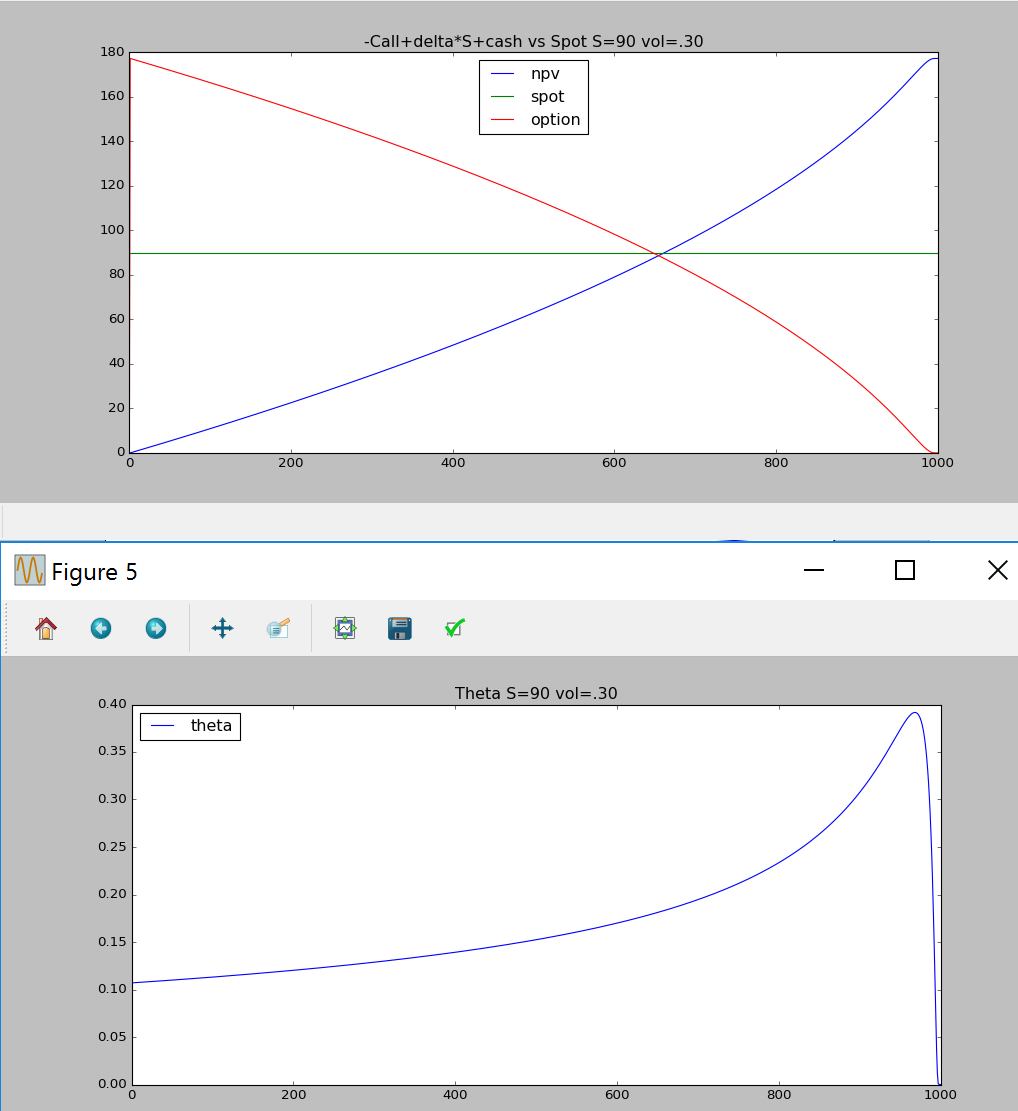
theta OTM delta hedging constant spot
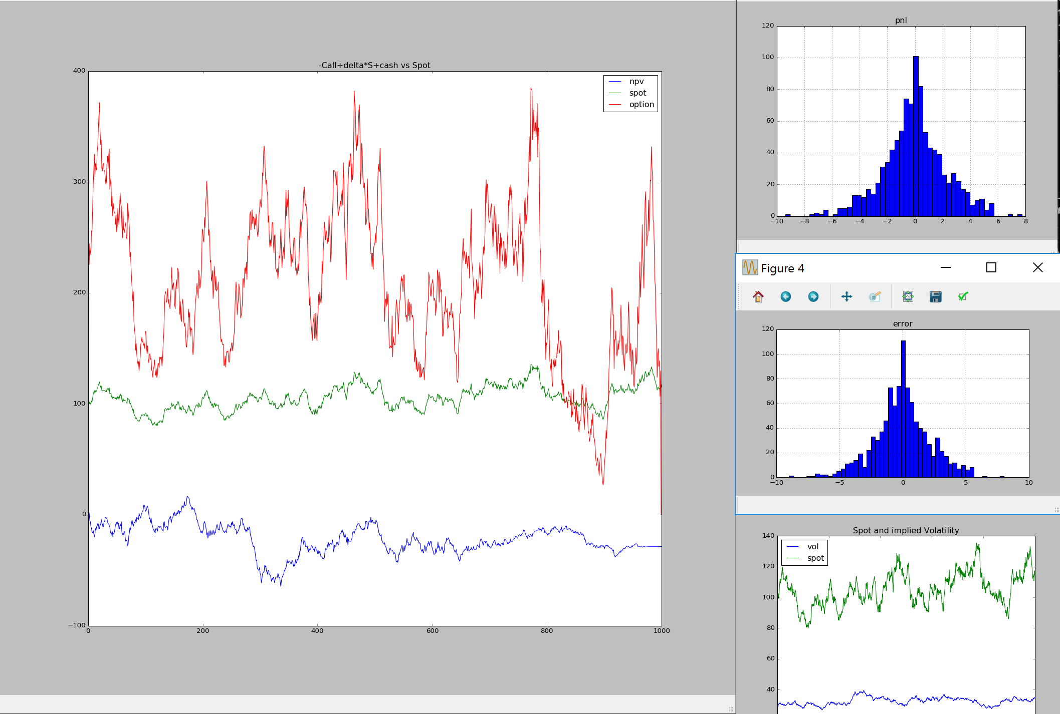
volaility dynamics
here we will run the code first on constant volaility , and then on stochastic implied volaility:
we can see that pnl has much wider distribution in the latter case. this is due to the fact that black sholes assumption does not hold anymore (we would need to hedge with other options to get better pnl profile)
constant vs stochastic volatility pnl delta hedging
import numpy as np
import pandas as pd
pd.set_option('display.width', 320)
pd.set_option('display.max_rows', 100)
pd.options.display.float_format = '{:,.2f}'.format
from scipy.stats import norm
import matplotlib.pyplot as plt

def BlackScholes(tau, S, K, sigma):
    d1=np.log(S/K)/sigma/np.sqrt(tau)+0.5*sigma*np.sqrt(tau)
    d2=d1-sigma*np.sqrt(tau)
    npv=(S*norm.cdf(d1)-K*norm.cdf(d2))
    delta=norm.cdf(d1)
    gamma=norm.pdf(d1)/(S*sigma*np.sqrt(tau))
    vega=S*norm.pdf(d1)*np.sqrt(tau)
    theta=-.5*S*norm.pdf(d1)*sigma/np.sqrt(tau)
    return {'npv':npv,'delta':delta,'gamma':gamma,'vega':vega,'theta':theta}

class Call(object):
    def __init__(self,start,T,K,N):
        self.T=T
        self.K=K
        self.start=start  #day to sell   option
        self.N=N

    def calc(self,today,vol,S):
        if today<self.start:
            return {'delta':0,'npv':0,'vega':0,'gamma':0,'theta':0,'intrinsic':0}
        if today>self.T:
            return {'delta':0,'npv':0,'vega':0,'gamma':0,'theta':0,'intrinsic':0}
        if today==self.T:
            return {'delta':0,'npv':0,'vega':0,'gamma':0,'theta':0,'intrinsic':self.N*max(0,S-self.K)}
        tau=(self.T-today)/250.
        call=BlackScholes(tau, S, self.K, vol)
        return {'delta':self.N*call['delta'],'npv':self.N*call['npv'],'vega':self.N*call['vega'],'gamma':self.N*call['gamma'],'theta':self.N*call['theta'],'intrinsic':self.N*max(0,S-self.K)}

def deltahedge(Ndays,Sdynamics="S*=(1.0+vol*np.sqrt(dt)*np.random.randn())",volDynamics="vol=.30"):
    S=90.0
    Strike=100.0
    vol=.30
    columns=('spot','vol','shares','cash','option','npv','vega','gamma','theta','pnlPredict')
    df = pd.DataFrame([[S,vol,0,0,0,0,0,0,0,0]],columns=columns)
    dt=1/250.
    cash=0
    dayToSellCall=1
    maturityCall=Ndays-1
    call=Call(dayToSellCall,maturityCall,Strike,-10)# sell one call on dayToSellCall day
    for day in xrange(1,Ndays+1):
        exec Sdynamics
        exec volDynamics

        if day==dayToSellCall: #sell call
          callValue=call.calc(day,vol,S)
          cash-=callValue['npv']

        #delta hedge
        callValue=call.calc(day,vol,S)
        delta=callValue['delta']
        currentNumberShares=df.iloc[day-1].shares
        sharesBuy=-currentNumberShares-delta
        cash-=sharesBuy*S
        if day==maturityCall:
            cash+=call.calc(day,vol,S)['intrinsic'] #settle call

        gamma=callValue['gamma']
        theta=callValue['theta']
        dS=S-df.iloc[day-1].spot
        pnlPredict=0.5*gamma*dS*dS+theta*dt
        dfnew=pd.DataFrame([[S,vol,-delta,cash,-callValue['npv'],cash+callValue['npv']-delta*S,callValue['vega'],gamma,theta/250.,pnlPredict]],columns=columns)
        df=df.append(dfnew,ignore_index=True)

    df['pnl'] = df['npv'] - df['npv'].shift(1)
    df['vol']=100.0*df['vol']
    df['error']=df['pnl']-df['pnlPredict']
    df.set_value(dayToSellCall, "error", 0)
    #df.loc[:,['vol','spot']].plot(title='Spot and implied Volatility')
    df.loc[:,['npv','spot','option']].plot(title='-Call+delta*S+cash vs Spot {0} {1}'.format(Sdynamics,volDynamics))
    df.loc[:,['theta']].plot(title='Theta {0} {1}'.format(Sdynamics,volDynamics))
    df.loc[:,['pnl']].hist(bins=50)
    #df.loc[:,['error']].hist(bins=50)
    print df.loc[:,['pnl']].describe()
    #print df

deltahedge(1000)#constant vol
deltahedge(1000,volDynamics="vol*=(1.0+0.5*np.sqrt(dt)*np.random.randn())")#stochastic vol
deltahedge(1000,Sdynamics="S=90") #consant OTM
deltahedge(10000,Sdynamics="S=100") #consant ATM
deltahedge(10000,Sdynamics="S=110")#consant ITM
deltahedge(10000,Sdynamics="S+=S*dt") #growing stock
plt.show()